We have set the task of minimizing the size of the box that encapsulates the update. According to this framework, the smallest conceivable box that still allows interaction between sites is one that encloses just two sites at a time. We define a new class of models with the following two properties: boxes encompass only pairs of sites (fig. 3), and every transaction is conservative. We will show that a useful model is possible even with the pairwise restriction. As a consequence, we will find that crystalline geometry is not necessary either. Such an update rule does not distinguish the neighbors from each other, in the way that (for example) a CA rule does (Fig. 3). It does not make use of the crystalline structure, and so can be applied to irregular lattices.
Conservation laws are fundamental in physics, and so they should be a part of a physical model. Local conservation also useful in dealing with the constraint of asynchrony and having only pairwise interactions. Global conservation will be achieved by construction: a certain variable or set of variables are designated as conserved quantities, and we design rules so that every local update leaves the sum of each conserved quantity over all sites unchanged.
One can thus think of the update as a ``transaction'' between sites. Periodically, a given pair of neighbors exchanges a packet of the conserved quantity; the loss from one is equal to the gain of the other. Each member of the pair then goes on to transact with other sites.
A simple example of the above class of models is a diffusion model, representing for example the diffusion of heat. We will call the conserved quantity q (representing the substance diffusing). A transaction between members of a pair transfers some of this quantity. In diffusion, the flux between two sites is proportional to the difference between them, so an appropriate rule is:
| (1) |
![]() so the transaction is
conservative. Figure 5 shows a time evolution of
this model.
so the transaction is
conservative. Figure 5 shows a time evolution of
this model.
As a more interesting example, we will simulate the physical phenomenon of waves. Waves are a ubiquitous phenomenon in physics, appearing in a variety of different systems - electromagnetic radiation and sound waves being two widely different examples that can nevertheless be described by the same kind of model.
All waves involve an amplitude associated with each point in space that changes over time. The future evolution of these amplitudes cannot be determined only from knowing all the amplitudes at a given moment. Travelling waves have a direction associated with them, and it is not possible to tell what the direction is by looking at an instantaneous snapshot; therefore they are an inherently second-order phenomenon. For this reason, the state of each site will be two quantities.
We choose momentum, p, as the conserved quantity. It will be shown that the system supports propagating waves in multiple dimensions, agreeing closely with the continuous wave equation, even when the sole possible interaction is two sites exchanging a packet of momentum. We will call the other quantity position, q (representing the amplitude of the wave).
In order to determine how much momentum two sites should exchange, we
associate a potential with a difference in q's between neighbors. We
can think of a site as a mass free to move in one dimension, connected
to its neighbors by springs. (Fig. 4) Two neighbors
exert a force (i.e., change in momentum) on each other which
depends on the displacement between them. Such a system is known to
support propagating waves and to be approximated by the scalar wave
equation
![]() .
Thus,
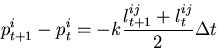
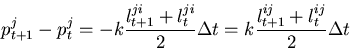
two sites i and j exchange momentum as follows:
.
Thus,
two sites i and j exchange momentum as follows:
| (2) |
| (3) |
Each site can now independently update its value of
q using its new value for p:
| (4) |
This system supports waves that can exhibit all the phenomena of continuous waves (Fig. 9), including reflection (Fig. 10) and refraction (Fig. 11). It also agrees quantitatively with a solution of the wave equation started from the same initial conditions, as shown in section 4.
In the above model, a difference in amplitude qi - qj between
neighbors can be considered to have potential energy; and p, because
it is directly related to a change in q, can be associated with
kinetic energy. Some of the potential energy converted into kinetic
energy, or vice versa, when an update happens. Since potentials only
make sense with pairs of sites, energy cannot be described for a
single site but only for a given pair. An obvious expression for the
total energy of a pair {i,j} of neighbors is
Designing a wave model that has a pairwise interaction rule that conserves this energy as well as momentum is more difficult than it may at first seem, for the following reason. Potential energy depends on a difference between two neighbors' amplitudes q, yet each site is potentially a member of many pairs, so changing q changes the potential energy in a way that depends on all neighbors simultaneously. So to conserve energy, it would seem necessary to know instantaneously the value of q of all the neighbors, and our box would have to enclose them as well. A site cannot avoid this problem by remembering the states of its neighbors: they may participate in other updates after this information is remembered but before it is used. The remembered state would therefore be out of date.
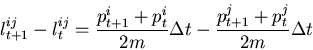
There is however a way to conserve energy with only pairwise interactions. We will abandon the idea of an absolute amplitude associated with each site, and instead associate a quantity with each pair of sites. Associated with the ``bond'' between two sites will be a quantity lij. This quantity alone will determine the potential energy, which is ``stored'' in the bond.1lij, instead of the relative position, will determine the potential and thus the momentum transfer between sites i and j. Its change is determined by the relative momenta of the two sites in the pair. It is now no longer possible to consider an absolute, scalar amplitude associated with each site such that the lij's are the differences between these amplitudes. The reason is that the lij's are decoupled from one another, unlike qi - qj.2
The update rule is somewhat more complicated in this case. To conserve energy, we use a leapfrog method [13] for the individual transaction. The leapfrog method advances each site a step at a time, but the position updates are a half step offset from the momentum updates:
 |
(6) |
 |
(7) |
 |
(8) |
Solving for the new values in terms of the old:
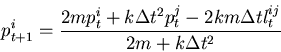 |
(9) |
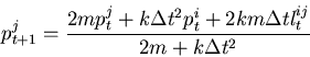 |
(10) |
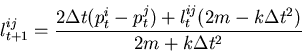 |
(11) |
We can write this a matrix T that transforms a vector of the old values of pi, pj, lij into the new ones:
![\begin{displaymath}
{1 \over 2m + k \Delta t^2}
\left[ \matrix{
2 m & k \Delta...
...r
2 \Delta t & -2 \Delta t & 2m - k \Delta t^2 \cr}
\right]
\end{displaymath}](img21.png) |
(12) |
As shown in figure 7, this system also exhibits all wave phenomena, and agrees quantitatively with the partial differential equation model as shown in section 4.