Figure: An example of an irregular lattice in two dimensions.

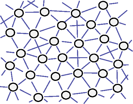Figure: A cluster of sites.

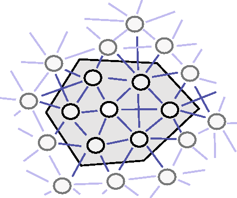Figure: A ``box'' enclosing a pair of neighbors.

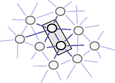Figure: Two neighboring sites exert a ``force'' on each other as if they were masses connected by springs. Each mass is free to move in one dimension.

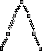Figure: Two-dimensional evolution of diffusion model. a=0.05, $\Delta t = 0.2$.

Figure: Superposition. a=0.05, $\Delta t = 0.01$, k = 1, neighborhood size variance = .0384. Sites are equally spaced but have variable sized neighborhoods. Above, the pulse is shown splitting into left-travelling and right-travelling pulses. Below, the pulses are shown after they have wrapped around the periodic boundary conditions and passed through each other twice, four times, and six times.

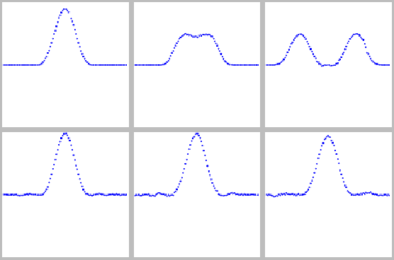Figure: A momentum wave in the energy-conserving wave model. The initial conditions are a pulse as in figure 6, and parameters are the same. There are 101 regularly spaced sites. Momentum rather than position is shown. The first four frame show the pulse in the process of splitting; the last shows it after one period. Energy was calculated to be identical before, during, and after the sequence, with a value of 0.33980601.

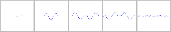Figure: Colors used in illustrations. Shades indicate amplitude from blue (-1) through white (0) to black (1).

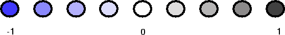Figure: Two-dimensional evolution of wave model. a=0.05, $\Delta t = 0.1$, k = 1.

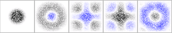Figure: Reflection. There is a parabola-shaped fixed boundary at right. The initial condition is a line wave, which becomes focused to a point in the third frame.

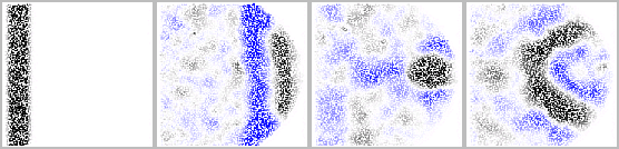Figure: Refraction. The central region has twice the density of sites as the rest of the space, but the neighborhood size remains about the same.

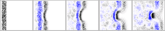Figure: Snapshot of amplitudes. As in Fig. 9 but with periodic boundary conditions.

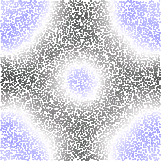Figure: Standing wave, comparison with exact solution. There are 101 processors arranged regularly in one dimension with two neighbors each; the graph shows the amplitude of the processor closest to the center plotted against average number of transactions per processor, versus the exact solution of the wave equation, $q(x,t) = sin(\pi x)cos(2 \pi t)$, with initial conditions $q(x,0) = sin(\pi x)$. a=0.05, $\Delta t = 0.05$, k = 1.

Figure: Comparison with solution of PDE: D(t) with exact solution over time for different levels of asynchrony a. The x-axis represents the average number of transactions per processor.

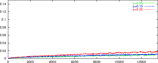Figure: Pulse, comparison D(t) with PDE solution. The sites are in one dimension with variable sized neighborhoods; the variance in neighborhood size is .0384. D(t) is plotted for regular and irregular geometry with 101 sites, and irregular geometry with 201 sites. In the first two, the pulse completed about two periods while in the last, it completed one period (a period being the time it takes the two halves of the pulse to wrap around the boundaries to their original starting points). a=0.05, $\Delta t = 0.01$, k = 1. The effect of irregularity is compensated for by using a greater density of sites.

Figure: As above, but normalized so that exactly two periods are completed in each case. The x-axis here represents periods.

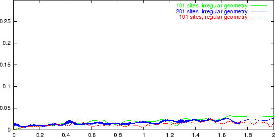Figure: Comparison with PDE solution D_p(t) for the momentum wave.