4. Simulation

We will now show a particular realization of the above class of discrete models. We will choose a particular method of placement of sites in space, and a particular rule for the occurrence of the updates. These will be chosen not for maximum efficiency; we will merely choose some conditions that satisfy the constraints outlined in section 2.

4.1 Asynchrony

We assume that the time between transactions for a given pair is approximately equal for all pairs. However, to make sure that updates are independent, our updating scheme should have the property that the pairings, when viewed globally, do not happen in the same order. (Otherwise, the identical order could be exploited to have the effect of synchronization.)

A scheme that meets these requirement is the following: let $\{\{i,j\}\vert j \in N\}$ be the set of pairs that include site i. Each pair in the set will update independently after an interval T(1 + X), where T is the period, X is a uniform random variable drawn from (-a,a) and $0 < a \ll 1$. This happens concurrently for all sites.

The above is described from a parallel point of view. Sequentially, the updating scheme can be viewed approximately as updating the pairs in a fixed order, with a small probability in each period for each pair to swap its spot in the schedule with a pair that is near it in time.

4.2 Irregular geometry

To test the model's lack of dependence on regular geometry, we need a lattice that is non-crystalline, but nevertheless ``spacelike''. This entails at least the following two conditions:

$\bullet$

Each site has about the same number of neighbors, with a low variance in the neighborhood size.

$\bullet$

Neighbors of a site have a high probability of being neighbors of each other.

Each site is assigned a Euclidean position randomly. For a site P, all processors within a radius r from P become P's neighbors, and each in turn has P as a neighbor.

A placement where all the coordinates are chosen at random leads roughly to a Poisson distribution of distances between sites, and therefore to a high variance in the number of neighbors. Instead, a distribution is chosen so that the average distance between connected sites will vary, but be close to some mean distance. This can be done by placing sites at random, but if two sites are too close to each other, eliminating one of them (see below).

An example of an irregular lattice in two dimensions produced as above is given in Fig. 1.

4.3 Realization

The models described here could be implemented on an amorphous computer [1] very straightforwardly. But as the first amorphous computers are just being built, and as we would like to test the effects of asynchrony and irregularity by varying them, it was necessary to simulate an amorphous computer on a sequential machine.

4.3.1 The Simulation environment: HLSIM

HLSIM [8] takes a single program in the high-level language Scheme [12] and simulates the execution of copies on thousands of asynchronous processors. Each processor can only communicate with some neighboring processors. Each has the ability to schedule local events in time using threads. HLSIM transforms these local events into a global schedule, and the order of events in this schedule is consistent with the order the events would fall in if each processor were running independently in parallel.

The connections between the processors can be specified in a geometric way. To satisfy the conditions given in section 4.2, the following algorithm was used:

$\bullet$

N_start sites are given a location in a Euclidean space using a Poisson distribution. That is, each coordinate is merely chosen uniformly from [0,1) at random.

$\bullet$

A site s is chosen at random. All sites within a distance r_min from s are deleted. This is repeated with a new randomly-chosen site until all remaining sites have been traversed. There are now no two processors within r_min of each other.

$\bullet$

For each site s, all sites within a radius r of s are connected tos.

This will eliminate some fraction 1 - d of the original sites which is a function of N_start and r_min. d was determined empirically in order to obtain a desired number of sites N_startd (accurate to within a few percent). An example of a lattice produced as above is shown in fig. 12.

The program run by each processor is very simple. A processor N₀ knows the identity of its neighbors, and for each neighbor N_i, it starts a separate thread i. This thread initially starts out by waiting for a random time drawn from [0,T). This is just to prevent the first transaction of every site from happening in a single instant. Then, a transaction takes place between N₀ and N_i, which causes the state of the pair Q(s₀,s_i) to be replaced by f(Q(s₀,s_i)). The transaction is assumed to be atomic. The processor waits for a time T + X, where X is a random variable drawn uniformly from [0, a). This is then repeated.⁴

The full source code is given in the appendix.

4.4 Observations

By starting the processors in some initial configuration and watching the evolution of the system, it becomes evident that the model supports all phenomena of linear waves. Fig. 6 demonstrates superposition, showing an initial pulse splitting into left-travelling and a right-travelling halves, which eventually wrap around the periodic boundary conditions and pass through each other unchanged.

Fig. 7 shows the same evolution for the energy-conserving model. Momentum is shown (since the model has no absolute position). The total energy over all pairs was computed at the beginning and various points during the evolution and found to be identical within the limits of machine precision, with a value of 0.33980601.

Figure 9 shows a time sequence of snapshots from a two-dimensional simulation with fixed boundary conditions. The initial condition is a sine-shaped perturbation in the center; a wave ripples out and reflects off the boundaries to interfere with itself. Various colors are used to indicate q, as shown in figure 8. There are about 5,000 processors, with an average neighborhood size of 6.365 and variance 1.133. Between the snapshots, each pair has made roughly 15 transactions. Figure 12 shows a single frame from a simulation with the same initial conditions, but with periodic boundary conditions.

In figure 10, the boundaries are fixed as in figure 9, except that the right boundary is shaped like a parabola. This is a ``mirror'' and the initial line wave is focused into a point.

By altering the properties of the interconnections, different ``media'' can be created for the waves to propagate through. In figure 11, there is also a line wave, but now there is a central region of more dense processors. Inside this region, the communication radius is shrunk so that the average number of neighbors is about the same as outside it. It thus has a different ``index of refraction'' than the rest of the medium and refracts the wave.

4.5 Quantitative comparisons

To test the model quantitatively and assess the effects of asynchrony and irregular geometry, we will compare its evolution to a solution to the continuous partial differential equation with the same initial conditions. Figures 13 through 17 show to what extent the model agrees with an exact solution of the continuous wave equation in one dimension:

$${d^2 q \over d t^2 } = c^2 { d^2 q \over d x^2 }.$$ (13)

with boundary conditions⁵ q(0,t) = 0 and q(1,t) = 0, and initial condition $q(x,0) = sin(\pi x)$. This equation has a solution

$$q(x,t) = sin(\pi x)cos(2 \pi t),$$ (14)

which is a standing wave. Figure 13 shows q for the processor closest to the center, plotted against a least-squares best fit of equation 14.

Figure 14 shows the difference of the model with the PDE with time for various levels of asynchrony a, plotted against average number of transactions per processor. 101 processors were arranged regularly with two neighbors each. Each site is given an initial value corresponding to $q(x,0) = sin(\pi x)$. That is, if x(s) is the Euclidean coordinate of site s, the initial coordinate is set to $sin(\pi x(s))$. Periodically, at time t, a measure D(t) of the local difference of q(s,t) with the PDE value at the corresponding time and location q_PDE(x(s),t) is computed and averaged over all sites. We used the square root of the average square of the difference, $D(t) = {1 \over \vert G\vert} \sqrt{\sum_{s \in G} [q_{PDE}(x(s)) - q(s)]^2}$, where G is the set of all sites. As with all comparisons of discrete and continuous models, the difference grows over time because there is some dispersion of the wave. Decreasing a below 0.15 does not have any appreciable effect.

The properties of wave propagation in the model were examined by setting the initial conditions to be a sinusoid pulse of width w:

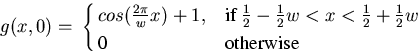$$g(x,0) = \hbox{ \cases{ cos({2 \pi \over w} x) + 1, &if ${... ... x < {1 \over 2} + {1 \over 2} w $\ \cr $0$\ &otherwise \cr} }$$ (15)

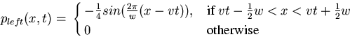
The wave equation with these initial conditions has as a solution the superposition of two pulses, one travelling left and the other travelling right:

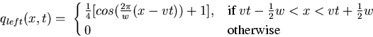$$q_{left}(x,t) = \hbox{ \cases{ {1 \over 4} [cos({2 \pi \ove... ...over 2} w < x < vt + {1 \over 2} w $\ \cr 0 &otherwise \cr} }$$ (16)

$$q_{right}(x,t) = \hbox{ \cases{ {1 \over 4} [cos({2 \pi \ov... ...\over 2} w < x < -vt + {1 \over 2} w$\ \cr 0 &otherwise \cr} }$$ (17)

Figure 15 shows the agreement of the model with the above solution; it plots the square root of the average square of the difference D(t) as above. D(t) is plotted for 101 sites and for 201 sites, versus number of transactions. With a greater density of sites, the wave propagates more slowly; figure 16 shows the same plot, but the x-axis is normalized so that two periods are completed in each case (a period being the time it takes the two halves of the pulse to wrap around the boundaries to their original starting points). With twice as many sites, disagreement with the PDE due to dispersion is significantly reduced. It is close to the disagreement for 101 sites with regular geometry. Thus we can compensate for the effects of irregularity by using a greater density of sites.

Figure 17 shows a comparison of the energy-conserving model to the PDE solution. It shows D_p(t) for 2 periods. D_p(t) is as D(t) but for momentum:

$D_p(t) = {1 \over \vert G\vert} \sqrt{\sum_{s \in G} [p_{PDE}(x(s)) - p(s)]^2}$. The model is compared to the solution of the PDE for momentum,

$$p_{left}(x,t) = \hbox{ \cases{ -{1 \over 4} sin({2 \pi \ove... ...over 2} w < x < vt + {1 \over 2} w $\ \cr 0 &otherwise \cr} }$$ (18)

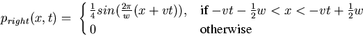$$p_{right}(x,t) = \hbox{ \cases{ {1 \over 4} sin({2 \pi \ove... ...\over 2} w < x < -vt + {1 \over 2} w$\ \cr 0 &otherwise \cr} }$$ (19)