

Next: Example: Partial differential
Up: Getting started: Programming
Previous: Getting started: Programming
Suppose we paint a surface with smart paint: We want the paint to
divide the surface into a few labeled regions, to identify the
boundaries between regions, and to generate a global data structure
that reflects the topology of how the regions are connected. This
region definition problem might be the first step in a program
that monitors the integrity of the structure that the paint covers, or
performs distributed control based on observing the local dynamical
variables.
In our imagined paint, there are enough computational elements that we
may think of them as particles that are randomly and uniformly
distributed throughout the paint. Each particle can communicate with
ten or twenty nearby neighbors, for example, through very short-range
radio or electrostatic communication, but a particle does not know the
directions or distances to its neighbors. (This is a conservative
assumption. Some hardware substrates may provide more geometric
information than this.) Each particle also has a hardware
random-number generator (not pseudo-random) that it can use to choose
an almost-unique identifier (the ID). We do not assume that there is
any a priori synchronization among particles.
To accomplish region definition, suppose that we are already at the
point where each particle has identified a set of neighbors with which
it can communicate. (Identifying the neighbors is already a
complicated part of the bootstrap process, but we will not talk about
it here.)
The first step is to do some small-scale local clustering. Each
particle initializes a state variable (its LOWNUM) to be that
particle's ID. The particle compares its LOWNUM to those of its
neighbors and adopts the smallest value as its new LOWNUM. This
process continues for a few iterations. At the end of this step we
have a few regions (particles that all have the same LOWNUM). Each
region has a radius approximately equal to the number of iterations,
but the regions are raggedly shaped, and they may have holes and
ill-defined boundaries.
The next step is to regularize the regions: smooth the edges and fill
in the holes. This can be done with a peer pressure algorithm.
Each particle computes a frequency table of the LOWNUMs of itself and
its neighbors, finds the LOWNUM that is asserted most often, and
adopts this as its new LOWNUM. This process continues until things
stabilize. Note that the LOWNUM for a region is in fact the particle
ID of a particular particle in that region. We can choose that
particle to act as a representative for the region.
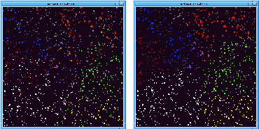
(Figure 1 shows an example of the algorithm in
progress.)

Figure 1: Progress of the region-growing
algorithm, from an initial configuration of 1000 particles placed at
random in a square of edge 1. Each particle's neighbors are all the
particles within a distance of of 0.1 from it. The picture on the
left shows the regions formed after local clustering but before
regularization. The figure on the right shows the effect of
regularization. Before regularization there are many regions and the
various regions are mixed together. Note how the regions become
compact and well-defined when regularized.
At this point the particles know whether they are interior to a
region, or on the boundaries between regions: Each particle notes all
the LOWNUMs asserted in its neighborhood. A particle that sees
more than one LOWNUM is near an edge. Particles that see
exactly two LOWNUMs are interior to the edge. More than two
LOWNUMs signals a vertex.
Now we use the same LOWNUM propagation algorithm, but restricted
to edges, so that each edge adopts a representative ID (and
associated particle). Each edge propagates to only those edges that
have the same two regions that they bound. Thus, disjoint edges that
bound the same two regions will be given different identifiers.
Now we do the same process for vertices, the particles at each vertex
pick an ID for the vertex (and a corresponding representative
particle).
Finally, we combine all this information by broadcast
accumulation. Each particle broadcasts what it knows: the IDs of the
regions, edges, and vertices, which edges separate which regions, and
which edges meet at each vertex. Initially, a particle knows only
about the structures it is a part of. But, as a particle receives
more information, it passes this along. To prevent saturation of
communication, a particle passes information along only when it learns
something new. Eventually, all particles will know all the
information.
This example is instructive in several ways:
- It exposes some common, useful patterns such as peer pressure
and comparison propagation.
- The ability for each region to pick a representative, although
not used above, is useful in establishing trees and communication
protocols.
- The algorithms tend to rely implicitly on geometry.
For example the regularization technique relies on assumptions about
rough uniform spatial distribution of the particles, and the fact that
peer-pressure will ``eat away'' at holes by filling in concavities.
The ideas here are reminiscent of computer vision algorithms, and some
of the techniques from computer vision may be relevant.

- We are organizing computational abstractions that will be
useful in controlling the behavior of the paint. For example we can
now regard the regions, edges, and vertices as computational objects
that have well-defined identities and known properties.


Next: Example: Partial differential
Up: Getting started: Programming
Previous: Getting started: Programming
Gerald Jay Sussman
Thu Jun 27 16:56:19 EDT 1996


