|
``In almost all textbooks, even the best, this principle is presented so that it is impossible to understand.'' (K. Jacobi, Lectures on Dynamics, 1842-1843). I have not chosen to break with tradition. V. I. Arnold, Mathematical Methods of Classical Mechanics [5], footnote, p. 246
|
There has been a remarkable revival of interest in classical mechanics in recent years. We now know that there is much more to classical mechanics than previously suspected. The behavior of classical systems is surprisingly rich; derivation of the equations of motion, the focus of traditional presentations of mechanics, is just the beginning. Classical systems display a complicated array of phenomena such as nonlinear resonances, chaotic behavior, and transitions to chaos.
Traditional treatments of mechanics concentrate most of their effort on the extremely small class of symbolically tractable dynamical systems. We concentrate on developing general methods for studying the behavior of systems, whether or not they have a symbolic solution. Typical systems exhibit behavior that is qualitatively different from the solvable systems and surprisingly complicated. We focus on the phenomena of motion, and we make extensive use of computer simulation to explore this motion.
Even when a system is not symbolically tractable, the tools of modern dynamics allow one to extract a qualitative understanding. Rather than concentrating on symbolic descriptions, we concentrate on geometric features of the set of possible trajectories. Such tools provide a basis for the systematic analysis of numerical or experimental data.
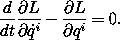
Classical mechanics is deceptively simple. It is surprisingly easy to get the right answer with fallacious reasoning or without real understanding. Traditional mathematical notation contributes to this problem. Symbols have ambiguous meanings that depend on context, and often even change within a given context.1 For example, a fundamental result of mechanics is the Lagrange equations. In traditional notation the Lagrange equations are written
The Lagrangian L must be interpreted as a function of the position
and velocity components qi and  i, so that the partial
derivatives make sense, but then in order for the time derivative
d/dt to make sense solution paths must have been inserted into the
partial derivatives of the Lagrangian to make functions of time. The
traditional use of ambiguous notation is convenient in simple
situations, but in more complicated situations it can be a serious
handicap to clear reasoning. In order that the reasoning be clear and
unambiguous, we have adopted a more precise mathematical notation.
Our notation is functional and follows that of modern mathematical
presentations.2
An introduction to our functional notation is in an appendix.
i, so that the partial
derivatives make sense, but then in order for the time derivative
d/dt to make sense solution paths must have been inserted into the
partial derivatives of the Lagrangian to make functions of time. The
traditional use of ambiguous notation is convenient in simple
situations, but in more complicated situations it can be a serious
handicap to clear reasoning. In order that the reasoning be clear and
unambiguous, we have adopted a more precise mathematical notation.
Our notation is functional and follows that of modern mathematical
presentations.2
An introduction to our functional notation is in an appendix.
Computation also enters into the presentation of the mathematical ideas underlying mechanics. We require that our mathematical notations be explicit and precise enough that they can be interpreted automatically, as by a computer. As a consequence of this requirement the formulas and equations that appear in the text stand on their own. They have clear meaning, independent of the informal context. For example, we write Lagrange's equations in functional notation as follows:3

The Lagrangian L is a real-valued function of time t,
coordinates x, and velocities v; the value is L(t, x, v). Partial
derivatives are indicated as derivatives of functions with respect to
particular argument positions;  2 L indicates the function
obtained by taking the partial derivative of the Lagrangian function
L with respect to the velocity argument position. The traditional
partial derivative notation, which employs a derivative with respect
to a ``variable,'' depends on context and can lead to ambiguity.4
The partial derivatives of the Lagrangian are then explicitly evaluated
along a path function q. The time derivative is taken and the
Lagrange equations formed. Each step is explicit; there are no
implicit substitutions.
2 L indicates the function
obtained by taking the partial derivative of the Lagrangian function
L with respect to the velocity argument position. The traditional
partial derivative notation, which employs a derivative with respect
to a ``variable,'' depends on context and can lead to ambiguity.4
The partial derivatives of the Lagrangian are then explicitly evaluated
along a path function q. The time derivative is taken and the
Lagrange equations formed. Each step is explicit; there are no
implicit substitutions.
Computational algorithms are used to communicate precisely some of the methods used in the analysis of dynamical phenomena. Expressing the methods of variational mechanics in a computer language forces them to be unambiguous and computationally effective. Computation requires us to be precise about the representation of mechanical and geometric notions as computational objects and permits us to represent explicitly the algorithms for manipulating these objects. Also, once formalized as a procedure, a mathematical idea becomes a tool that can be used directly to compute results.
Active exploration on the part of the student is an essential part of the learning experience. Our focus is on understanding the motion of systems; to learn about motion the student must actively explore the motion of systems through simulation and experiment. The exercises and projects are an integral part of the presentation.
That the mathematics is precise enough to be interpreted automatically allows active exploration to be extended to it. The requirement that the computer be able to interpret any expression provides strict and immediate feedback as to whether the expression is correctly formulated. Experience demonstrates that interaction with the computer in this way uncovers and corrects many deficiencies in understanding.
In this book we express computational methods in Scheme, a dialect of the Lisp family of programming languages that we also use in our introductory computer science subject at MIT. There are many good expositions of Scheme. We provide a short introduction to Scheme in an appendix.
Even in the introductory computer science class we never formally teach the language, because we do not have to. We just use it, and students pick it up in a few days. This is one great advantage of Lisp-like languages: They have very few ways of forming compound expressions, and almost no syntactic structure. All of the formal properties can be covered in an hour, like the rules of chess. After a short time we forget about the syntactic details of the language (because there are none) and get on with the real issues -- figuring out what we want to compute.
The advantage of Scheme over other languages for the exposition of classical mechanics is that the manipulation of procedures that implement mathematical functions is easier and more natural in Scheme than in other computer languages. Indeed, many theorems of mechanics are directly representable as Scheme programs.
The version of Scheme that we use in this book is MIT Scheme, augmented with a large library of software called Scmutils that extends the Scheme operators to be generic over a variety of mathematical objects, including symbolic expressions. The Scmutils library also provides support for the numerical methods we use in this book, such as quadrature, integration of systems of differential equations, and multivariate minimization.
The Scheme system, augmented with the Scmutils library, is free
software. We provide this system, complete with documentation and
source code, in a form that can be used with the GNU/Linux operating
system, on the Internet at
http://www-mitpress.mit.edu/sicm.
This book presents classical mechanics from an unusual perspective. It focuses on understanding motion rather than deriving equations of motion. It weaves recent discoveries in nonlinear dynamics throughout the presentation, rather than presenting them as an afterthought. It uses functional mathematical notation that allows precise understanding of fundamental properties of classical mechanics. It uses computation to constrain notation, to capture and formalize methods, for simulation, and for symbolic analysis.
This book is the result of teaching classical mechanics at MIT for the past six years. The contents of our class began with ideas from a class on nonlinear dynamics and solar system dynamics by Wisdom and ideas about how computation can be used to formulate methodology developed in an introductory computer science class by Abelson and Sussman. When we started we expected that using this approach to formulate mechanics would be easy. We quickly learned that many things we thought we understood we did not in fact understand. Our requirement that our mathematical notations be explicit and precise enough that they can be interpreted automatically, as by a computer, is very effective in uncovering puns and flaws in reasoning. The resulting struggle to make the mathematics precise, yet clear and computationally effective, lasted far longer than we anticipated. We learned a great deal about both mechanics and computation by this process. We hope others, especially our competitors, will adopt these methods, which enhance understanding while slowing research.
1 In his book on mathematical pedagogy [17], Hans Freudenthal argues that the reliance on ambiguous, unstated notational conventions in such expressions as f(x) and df(x)/dx makes mathematics, and especially introductory calculus, extremely confusing for beginning students; and he enjoins mathematics educators to use more formal modern notation.
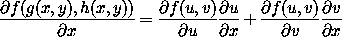
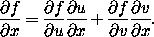
2 In his beautiful book Calculus on Manifolds [40], Michael Spivak uses functional notation. On p. 44 he discusses some of the problems with classical notation. We excerpt a particularly juicy passage:
The mere statement of [the chain rule] in classical notation requires the introduction of irrelevant letters. The usual evaluation for D1(fo(g,h)) runs as follows:If f(u,v) is a function and u = g(x,y) and v = h(x,y) then
[The symbol
Note that f means something different on the two sides of the equation!
3 This is presented here without explanation, to give the flavor of the notation. The text gives a full explanation.
4 ``It is necessary to use the apparatus of partial derivatives, in which even the notation is ambiguous.'' V.I. Arnold, Mathematical Methods of Classical Mechanics [5], Section 47, p. 258. See also the footnote on that page.