 = m
= m .
.
Lagrange's equations are a system of second-order differential
equations. In order to use them to compute the evolution of a
mechanical system, we must find a suitable Lagrangian for the system.
There is no general way to construct a Lagrangian for every system,
but there is an important class of systems for which we can identify
Lagrangians in a straightforward way in terms of kinetic and potential
energy. The key idea is
to construct a Lagrangian L such that Lagrange's equations are
Newton's equations = m.
Suppose our system consists of N
particles indexed by  , with mass m and vector
position
, with mass m and vector
position  (t). Suppose further that the forces acting
on the particles can be written in terms of a gradient of a
potential energy
(t). Suppose further that the forces acting
on the particles can be written in terms of a gradient of a
potential energy  that is a function of the positions of the
particles and possibly time, but does not depend on the
velocities. In other words, the force on particle is
= -
that is a function of the positions of the
particles and possibly time, but does not depend on the
velocities. In other words, the force on particle is
= -  , where
is the gradient of with
respect to the position of the particle with index . We can
write Newton's equations as
, where
is the gradient of with
respect to the position of the particle with index . We can
write Newton's equations as

Vectors can be represented as tuples of components of the vectors on a
rectangular basis. So 1(t) is represented as the tuple
x1(t). Let V be the potential energy function
expressed in terms of components:


where  1, V is the partial derivative of V with
respect to the x(t) argument slot.
1, V is the partial derivative of V with
respect to the x(t) argument slot.
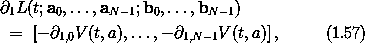
To form the Lagrange equations we collect all the position components of all the particles into one tuple x(t), so x(t) = (x0(t), ..., xN-1(t)). The Lagrange equations for the coordinate path x are

Observe that Newton's equations (1.51) are just the components of the Lagrange equations (1.54) if we choose L to have the properties

here
V(t, x(t)) = V(t; x0(t), ..., xN-1(t))
and
1, V(t, x(t)) is the tuple of the
components of the derivative of V with respect to the coordinates of
the particle with index , evaluated at time t and
coordinates x(t).
These conditions are satisfied if for every a and b

where a = (a0, ... , aN-1). We use the symbols a and b to emphasize that these are just formal parameters of the Lagrangian. One choice for L that has the required properties (1.56-1.57) is

where v2 is the sum of the squares of the components of
v.61
The first term is the kinetic energy, conventionally denoted T. So this choice for the Lagrangian is L(t, x, v) = T(t, x, v) - V(t, x), the difference of the kinetic and potential energy. We will often extend the arguments of the potential energy function to include the velocities so that we can write L = T - V.62
Given a system of point particles for which we can identify the force as the (negative) derivative of a potential energy V that is independent of velocity, we have shown that the system evolves along a path that satisfies Lagrange's equations with L = T - V. Having identified a Lagrangian for this class of systems, we can restate the principle of stationary action in terms of energies. This statement is known as Hamilton's principle: A point-particle system for which the force is derived from a velocity-independent potential energy evolves along a path q for which the action

is stationary with respect to variations of the path q that leave the endpoints fixed, where L = T - V is the difference between kinetic and potential energy.63
It might seem that we have reduced Lagrange's equations to nothing
more than = m , and indeed, the principle is
motivated by comparing the two equations for this special class of
systems. However, the Lagrangian formulation of the equations of
motion has an important advantage over = m . Our
derivation used the rectangular components x of
the positions of the constituent particles for the generalized
coordinates, but if the system's path satisfies Lagrange's equations
in some particular coordinate system, it must satisfy the equations in
any coordinate system. Thus we see that L = T - V is suitable as
a Lagrangian with any set of generalized coordinates. The
equations of variational mechanics are derived the same way in any
configuration space and any coordinate system. In contrast, the
Newtonian formulation is based on elementary geometry: In order for
D2(t) to be meaningful as an acceleration, (t) must
be a vector in physical space. Lagrange's equations have no such
restriction on the meaning of the coordinate q. The generalized
coordinates can be any parameters that conveniently describe the
configurations of the system.
Consider a particle of mass m in a uniform gravitational field with acceleration g. The potential energy is m g h where h is the height of the particle. The kinetic energy is just (1/2) mv2. A Lagrangian for the system is the difference of the kinetic and potential energies. In rectangular coordinates, with y measuring the vertical position and x measuring the horizontal position, the Lagrangian is L(t; x, y; vx, vy) = (1/2) m ( vx2 + vy2 ) - m g y. We have64
(define ((L-uniform-acceleration m g) local)
(let ((q (coordinate local))
(v (velocity local)))
(let ((y (ref q 1)))
(- (* 1/2 m (square v)) (* m g y)))))
(show-expression
(((Lagrange-equations
(L-uniform-acceleration 'm 'g))
(up (literal-function 'x)
(literal-function 'y)))
't))

This equation describes unaccelerated motion in the horizontal direction (mD2 x(t) = 0) and constant acceleration in the vertical direction (mD2 y(t) = - g m).
Consider planar motion of a particle of mass m in a central force field, with an arbitrary potential energy U(r) depending only upon the distance r to the center of attraction. We will derive the Lagrange equations for this system in both rectangular coordinates and polar coordinates.
In rectangular coordinates (x, y), with origin at the center of attraction, the potential energy is V(t; x, y) = U((x2 + y2)1/2) and the kinetic energy is T(t; x, y; vx, vy) = (1/2) m (vx2 + vy2). A Lagrangian for the system is L = T - V:

As a procedure:
(define ((L-central-rectangular m U) local)
(let ((q (coordinate local))
(v (velocity local)))
(- (* 1/2 m (square v))
(U (sqrt (square q))))))
The Lagrange equations are
(show-expression
(((Lagrange-equations
(L-central-rectangular 'm (literal-function 'U)))
(up (literal-function 'x)
(literal-function 'y)))
't))

We can rewrite these Lagrange equations as:

where r(t) = ((x(t))2 + (y(t))2)1/2. We can interpret these as follows. The particle is subject to a radially directed force with magnitude - DU(r). Newton's equations equate the force with the product of the mass and the acceleration. The two Lagrange equations are just the rectangular components of Newton's equations.
We can describe the same system in polar coordinates.
The relationship between rectangular coordinates (x, y) and polar
coordinates (r,  ) is
) is

The relationship of the generalized velocities is derived from the
coordinate transformation. Consider a configuration path that is
represented in both rectangular and polar coordinates. Let
 and
and  be components of the rectangular
coordinate path, and let
be components of the rectangular
coordinate path, and let  and
and  be
components of the corresponding polar coordinate path. The
rectangular components at time t are ((t),
(t)) and the polar coordinates at time t are
((t), (t)). They are related
by (1.62):
be
components of the corresponding polar coordinate path. The
rectangular components at time t are ((t),
(t)) and the polar coordinates at time t are
((t), (t)). They are related
by (1.62):

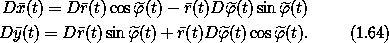
The rectangular
velocity at time t is (D(t), D(t)).
Differentiating (1.63) gives the
relationship among the velocities
These relations are valid for any configuration path at any moment, so
we can abstract them to relations among coordinate representations of
an arbitrary velocity. Let vx and vy be the rectangular
components of the velocity and  and
and  be the
rate of change of r and . Then
be the
rate of change of r and . Then

The kinetic energy is (1/2) m(vx2 + vy2):


We express this Lagrangian as follows:
(define ((L-central-polar m U) local)
(let ((q (coordinate local))
(qdot (velocity local)))
(let ((r (ref q 0)) (phi (ref q 1))
(rdot (ref qdot 0)) (phidot (ref qdot 1)))
(- (* 1/2 m
(+ (square rdot)
(square (* r phidot))) )
(U r)))))
(show-expression
(((Lagrange-equations
(L-central-polar 'm (literal-function 'U)))
(up (literal-function 'r)
(literal-function 'phi)))
't))

We can interpret the first equation as saying that the product of
the mass and the radial acceleration is the sum of the force due to
the potential and the centrifugal force. The second equation can be
interpreted as saying that the derivative of the angular momentum
mr2D is zero, so angular momentum is conserved.
Note that we used the same Lagrange-equations procedure for the derivation in both coordinate systems. Coordinate representations of the Lagrangian are different for different coordinate systems, and the Lagrange equations in different coordinate systems look different. Yet the same method is used to derive the Lagrange equations in any coordinate system.
Check that the Lagrange equations for central force motion in polar coordinates and in rectangular coordinates are equivalent. Determine the relationship among the second derivatives by substituting paths into the transformation equations and computing derivatives, then substitute these relations into the equations of motion.
The motion of a system is independent of the coordinates we use to describe it. This coordinate-free nature of the motion is apparent in the action principle. The action depends only on the value of the Lagrangian along the path and not on the particular coordinates used in the representation of the Lagrangian. We can use this property to find a Lagrangian in one coordinate system in terms of a Lagrangian in another coordinate system.
Suppose we have a mechanical system whose motion is described by a Lagrangian L that depends on time, coordinates, and velocities. And suppose we have a coordinate transformation F such that x = F(t, x'). The Lagrangian L is expressed in terms of the unprimed coordinates. We want to find a Lagrangian L' expressed in the primed coordinates that describes the same system. One way to do this is to require that the value of the Lagrangian along any configuration path be independent of the coordinate system. If q is a path in the unprimed coordinates and q' is the corresponding path in primed coordinates, then the Lagrangians must satisfy:

We have seen that the transformation from rectangular to polar coordinates implies that the generalized velocities transform in a certain way. The velocity transformation can be deduced from the requirement that a path in polar coordinates and a corresponding path in rectangular coordinates are consistent with the coordinate transformation. In general, the requirement that paths in two different coordinate systems be consistent with the coordinate transformation can be used to deduce how all of the components of the local tuple transform. Given a coordinate transformation F, let C be the corresponding function that maps local tuples in the primed coordinate system to corresponding local tuples in the unprimed coordinate system:

We will deduce the general form of C below.
Given such a local-tuple transformation C, a Lagrangian L' that satisfies equation (1.68) is

We can see this by substituting for L' in equation (1.68):

To find the local-tuple transformation C given a coordinate transformation F, we deduce how each component of the local tuple transforms. Of course, the coordinate transformation specifies how the coordinate component of the local tuple transforms. The generalized-velocity component of the local-tuple transformation can be deduced as follows. Let q and q' be the same configuration path expressed in the two coordinate systems. Substituting these paths into the coordinate transformation and computing the derivative, we find

Through any point there is always a path of any given velocity, so we may generalize and conclude that along corresponding coordinate paths the generalized velocities satisfy

If needed, rules for higher-derivative components of the local tuple can be determined in a similar fashion. The local-tuple transformation that takes a local tuple in the primed system to a local tuple in the unprimed system is constructed from the component transformations:

So if we take the Lagrangian L' to be

then the action has a value that is independent of the coordinate system used to compute it. The configuration path of stationary action does not depend on which coordinate system is used to describe the path. The Lagrange equations derived from these Lagrangians will in general look very different from one another, but they must be equivalent.
Exercise 1.14.
Show by direct calculation that the Lagrange equations for L' are
satisfied if the Lagrange equations for L are satisfied.
Given a coordinate transformation F, we can use (1.74) to find the function C that transforms local tuples. The procedure F->C implements this:65
(define ((F->C F) local)
(->local (time local)
(F local)
(+ (((partial 0) F) local)
(* (((partial 1) F) local)
(velocity local)))))
As an illustration, consider the transformation from polar to
rectangular coordinates, x = r cos and y = r sin ,
with the following implementation:
(define (p->r local)
(let ((polar-tuple (coordinate local)))
(let ((r (ref polar-tuple 0))
(phi (ref polar-tuple 1)))
(let ((x (* r (cos phi)))
(y (* r (sin phi))))
(up x y)))))
In terms of the polar coordinates and the rates of change of the polar coordinates, the rates of change of the rectangular components are
(show-expression
(velocity
((F->C p->r)
(->local 't (up 'r 'phi) (up 'rdot 'phidot)))))

We can use F->C to find the Lagrangian for central force motion in polar coordinates from the Lagrangian in rectangular components, using equation (1.70):
(define (L-central-polar m U)
(compose (L-central-rectangular m U) (F->C p->r)))
(show-expression
((L-central-polar 'm (literal-function 'U))
(->local 't (up 'r 'phi) (up 'rdot 'phidot))))

The result is the same as Lagrangian (1.67).
Exercise 1.15. Central force motion
Find Lagrangians for central force motion in three dimensions in
rectangular coordinates and in spherical coordinates. First, find the
Lagrangians analytically, then check the results with the computer by
generalizing the programs that we have presented.
We have found that L = T - V is a suitable Lagrangian for a system of point particles subject to forces derived from a potential. Extended bodies can sometimes be conveniently idealized as a system of point particles connected by rigid constraints. We will find that L = T - V, expressed in irredundant coordinates, is a suitable Lagrangian for modeling systems of point particles with rigid constraints. We will first illustrate the method and then provide a justification.
The system is presumed to be made of N point masses, indexed by ,
in ordinary three-dimensional space. The first step is to
choose a convenient set of irredundant generalized coordinates q and
redescribe the system in terms of these. In terms of the generalized
coordinates the rectangular coordinates of particle are

For irredundant coordinates q all the coordinate constraints are
built into the functions f.
We deduce the relationship of the generalized velocities v to the
velocities of the constituent particles v by
inserting path functions into
equation (1.76),
differentiating, and abstracting to arbitrary velocities.66
We find

We use equations (1.76) and
(1.77) to
express the kinetic energy in terms of the generalized coordinates and
velocities.
Let  be the kinetic energy as a function of the
rectangular coordinates and velocities:
be the kinetic energy as a function of the
rectangular coordinates and velocities:

where v2 is the squared magnitude of v.
As a function of the generalized coordinate tuple q and the
generalized velocity tuple v, the kinetic energy is

Similarly, we use
equation (1.76) to reexpress
the potential energy in terms of the generalized coordinates. Let
 (t, x) be the potential energy at time t in the
configuration specified by the tuple of rectangular coordinates x.
Expressed in generalized coordinates the potential energy is
(t, x) be the potential energy at time t in the
configuration specified by the tuple of rectangular coordinates x.
Expressed in generalized coordinates the potential energy is

We take the Lagrangian to be the difference of the kinetic energy and the potential energy: L = T - V.
Consider a pendulum (see figure 1.2) of length l and mass m, modeled as a point mass, supported by a pivot that is driven in the vertical direction by a given function of time ys.

The dimension of the configuration space for this system is one; we
choose  , shown in figure 1.2, as the
generalized coordinate.
, shown in figure 1.2, as the
generalized coordinate.
The position of the bob is given, in rectangular coordinates, by


obtained by differentiating along a path and abstracting to velocities at the moment.
The kinetic energy is (t; x, y; vx, vy) = (1/2) m
(vx2 + vy2). Expressed in generalized coordinates the kinetic
energy is

The potential energy is (t; x, y) = mgy. Expressed in
generalized coordinates the potential energy is

The Lagrangian is expressed as
(define ((T-pend m l g ys) local)
(let ((t (time local))
(theta (coordinate local))
(thetadot (velocity local)))
(let ((vys (D ys)))
(* 1/2 m
(+ (square (* l thetadot))
(square (vys t))
(* 2 l (vys t) thetadot (sin theta)))))))
(define ((V-pend m l g ys) local)
(let ((t (time local))
(theta (coordinate local)))
(* m g (- (ys t) (* l (cos theta))))))
(define L-pend (- T-pend V-pend))
Lagrange's equation for this system is67
(show-expression
(((Lagrange-equations
(L-pend 'm 'l 'g (literal-function 'y_s)))
(literal-function 'theta))
't))

Exercise 1.16.
Derive the Lagrangians in exercise 1.9.
Exercise 1.17. Bead on a helical wire
A bead of mass m is constrained to move on a frictionless helical
wire. The helix is oriented so that its axis is horizontal. The
diameter of the helix is d and its pitch (turns per unit length) is
h. The system is in a uniform gravitational field with vertical acceleration
g. Formulate a Lagrangian that describes the system and find the
Lagrange equations of motion.
Exercise 1.18. Bead on a triaxial surface
A bead of mass m moves without friction on a triaxial ellipsoidal
surface. In rectangular coordinates the surface satisfies

for some constants a, b, and c. Identify suitable generalized coordinates, formulate a Lagrangian, and find Lagrange's equations.
Exercise 1.19. A two-bar linkage
The two-bar linkage shown in figure 1.3 is constrained to
move in the plane. It is composed of three small massive bodies
interconnected by two massless rigid rods in a uniform gravitational
field with vertical acceleration g.
The rods are pinned to the central body
by a hinge that allows the linkage to fold. The
system is arranged so that the hinge is completely free: the members
can go through all configurations without collision. Formulate a
Lagrangian that describes the system and find the Lagrange equations
of motion. Use the computer to do this, because the equations are
rather big.

Exercise 1.20. Sliding pendulum
Consider a pendulum of length l attached to a support that is free
to move horizontally, as shown in figure 1.4.
Let the mass of the support be m1 and the
mass of the pendulum be m2.
Formulate a Lagrangian and derive Lagrange's equations for this
system.

In this section we show that L = T - V is in fact a suitable Lagrangian for rigidly constrained systems. We do this by requiring that the Lagrange equations be equivalent to the Newtonian vectorial dynamics with vector constraint forces.68
We consider a system of particles. The particle with index
has mass m and position (t) at time t. There may be a
very large number of these particles, or just a few. Some of the
positions may also be specified functions of time, such as the position of
the pivot of a driven pendulum.
There are rigid position
constraints among some of the particles. We assume that all of these
constraints are of the form

that is, the distance between particles and ß is lß.
The Newtonian equation of motion for particle says that
the mass times the acceleration of particle is equal to the
sum of the potential forces and the constraint forces. The potential
forces are derived as the negative gradient of the potential energy,
and may depend on the positions of the other particles and the time.
The constraint forces ß are the vector
constraint forces associated with the rigid constraint between
particle and particle ß. So

where in the summation ß ranges over only those particle
indices for which there are rigid constraints with the particle
indexed by ; we use the notation ß <-->
for the relation that there is a rigid constraint between the
indicated particles.
The force of constraint is directed along the line between the particles, so we may write

where Fß(t) is the scalar magnitude of the tension in the
constraint at time t. Note that ß = -
ß. In general, the scalar constraint forces
change as the system evolves.
Formally, we can reproduce Newton's equations with the Lagrangian69
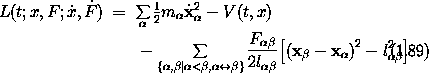
where the constraint forces are being treated as additional
generalized coordinates. Here x is a structure composed of all
the rectangular components x of all the
,  is a structure composed of all the
rectangular components
is a structure composed of all the
rectangular components  of all the
velocity vectors
of all the
velocity vectors  , and F is a structure composed of
all the Fß. The velocity of
F does not appear in the Lagrangian, and F itself appears only
linearly. So the Lagrange equations associated with F are
, and F is a structure composed of
all the Fß. The velocity of
F does not appear in the Lagrangian, and F itself appears only
linearly. So the Lagrange equations associated with F are

but this is just a restatement of the constraints. The Lagrange equations for the coordinates of the particles are Newton's equations (1.87)

Now that we have a suitable Lagrangian, we can use the fact that Lagrangians can be reexpressed in any generalized coordinates to find a simpler Lagrangian. The strategy is to choose a new set of coordinates for which many of the coordinates are constants and the remaining coordinates are irredundant.
Let q be a tuple of generalized coordinates that specify the degrees of freedom of the system without redundancy. Let c be a tuple of other generalized coordinates that specify the distances between particles for which constraints are specified. The c coordinates will have constant values. The combination of q and c replaces the redundant rectangular coordinates x.70 In addition, we still have the F coordinates, which are the scalar constraint forces. Our new coordinates are the components of q, c, and F.
There exist functions f that give the rectangular
coordinates of the constituent particles in terms of q and c:

To reexpress the Lagrangian in terms of q, c, and F, we need to find
v in terms of the generalized velocities
 and
and  : we do this by differentiating f
along a path and abstracting to arbitrary velocities (see
section 1.6.1):
: we do this by differentiating f
along a path and abstracting to arbitrary velocities (see
section 1.6.1):

Substituting these into Lagrangian (1.89), and using

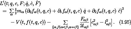
The Lagrange equations are derived by the usual procedure. Rather than write out all the gory details, let's think about how it will go.
The Lagrange equations associated with F just restate the constraints:

and consequently we know that along a solution path, c(t) = l and Dc(t) = D2c(t) = 0. We can use this result to simplify the Lagrange equations associated with q and c.
The Lagrange equations associated with q are the same as if they were derived from the Lagrangian71

but this is exactly T - V where T and V are computed from the generalized coordinates q, with fixed constraints. Notice that the constraint forces do not appear in the Lagrange equations for q because in the Lagrange equations they are multiplied by a term that is identically zero on the solution paths. So the Lagrange equations for T - V with irredundant generalized coordinates q and fixed constraints are equivalent to Newton's equations with vector constraint forces.
The Lagrange equations for c can be used to find the constraint forces. The Lagrange equations are a big mess so we will not show them explicitly, but in general they are equations in D2c, Dc, and c that will depend upon q, Dq, and F. The dependence on F is linear, so we can solve for F in terms of the solution path q and Dq, with c = l and Dc = D2c = 0.
If we are not interested in the constraint forces, we can abandon the full Lagrangian (1.95) in favor of Lagrangian (1.97), which is equivalent as far as the evolution of the generalized coordinates q is concerned.
The same derivation goes through even if the lengths
lß specified in the interparticle distance
constraints are a function of time. It can also be generalized to
allow distance constraints to time-dependent positions, by making some
of the positions of particles ß be specified functions of
time.
Consider a constraint of the form

where x(t) is the structure of all the rectangular components x(t) at time t.
In section 1.10 we will show, using the
variational principle, that an
appropriate Lagrangian for this system is

where  is an additional coordinate and
  is the
corresponding generalized velocity.
The Lagrange equations associated with are just a
restatement of the constraints: (t, x(t)) = 0 .
The Lagrange equations for the particle coordinates are
is the
corresponding generalized velocity.
The Lagrange equations associated with are just a
restatement of the constraints: (t, x(t)) = 0 .
The Lagrange equations for the particle coordinates are

Such a constraint can also be modeled by including appropriate constraint forces in Newton's equations:

For
equations (1.100)
to be the same as
equations (1.101) we
must identify (t) 1, (t, x(t)) with the
forces of constraint on particle . Notice that these forces
of constraint are proportional to the normal to the constraint surface
at each instant and thus do no work for motions that obey the
constraint.
Lagrangian (1.89), which we developed above to
include Newtonian forces of constraint for position constraints, is of exactly
this form. We can identify

The forces of constraint satisfy

Accepting
Lagrangian (1.99) as
describing systems with constraints of the
form (1.98), we can make a coordinate
transformation from the redundant
coordinates x to irredundant generalized coordinates q and
constraint coordinates c = (t,x), as above. The coordinate
will not appear in the Lagrange equations for q because on
solution paths they will be multiplied by a factor that is identically
zero. If we are interested only in the evolution of the generalized
coordinates, we can assume the constraints are identically satisfied
and take the Lagrangian to be the difference of the
kinetic and potential energies expressed in terms of the generalized
coordinates.

Exercise 1.21. The dumbbell
In this exercise we will recapitulate the derivation of the Lagrangian
for constrained systems for a particular simple system.
Consider two massive particles in the plane constrained by a massless rigid rod to remain a distance l apart, as in figure 1.5. There are apparently four degrees of freedom for two massive particles in the plane, but the rigid rod reduces this number to three.
We can uniquely specify the configuration with the redundant coordinates of the particles, say x0(t), y0(t) and x1(t), y1(t). The constraint (x1(t) - x0(t))2 + (y1(t) - y0(t))2 = l2 eliminates one degree of freedom.
a. Write Newton's equations for the balance of forces for the four rectangular coordinates of the two particles, given that the scalar tension in the rod is F.
b. Write the formal Lagrangian

such that Lagrange's equations will yield the Newton's equations you derived in part a.
c. Make a change of coordinates to a coordinate system with
center of mass coordinates xcm, ycm, angle ,
distance between the particles c, and tension force F. Write the
Lagrangian in these coordinates, and write the Lagrange equations.
d. You may deduce from one of these equations that c(t) = l. From
this fact we get that Dc = 0 and D2c = 0. Substitute these into the
Lagrange equations you just computed to get the equation of motion for
xcm, ycm, .
e. Make a Lagrangian ( = T - V) for the system described with the
irredundant generalized coordinates xcm, ycm,
and compute the Lagrange equations from this Lagrangian. They should
be the same equations as you derived for the same coordinates in
part d.
Exercise 1.22. Driven pendulum
Show that the Lagrangian (1.89) can be used to
describe the driven pendulum, where the position of the pivot is a
specified function of time: Derive the equations of motion using the
Newtonian constraint force prescription, and show that they are the
same as the Lagrange equations. Be sure to examine the equations for
the constraint forces as well as the position of the pendulum bob.
Exercise 1.23. Fill in the details
Show that the Lagrange equations for
Lagrangian (1.97) are the same
as the Lagrange equations for
Lagrangian (1.95) with the
substitution c(t) = l, Dc(t) = D2c(t) = 0.
Exercise 1.24. Constraint forces
Find the tension in an undriven planar pendulum.
The derivation of a Lagrangian for a constrained system involves steps that are analogous to those in the derivation of a coordinate transformation.
For a constrained system we specify the rectangular coordinates of the constituent particles in terms of generalized coordinates that incorporate the constraints. We then determine the rectangular velocities of the constituent particles as functions of the generalized coordinates and the generalized velocities. The Lagrangian that we know how to express in rectangular coordinates and velocities of the constituent particles can then be reexpressed in terms of the generalized coordinates and velocities.
To carry out a coordinate transformation one specifies how the configuration of a system expressed in one set of generalized coordinates can be reexpressed in terms of another set of generalized coordinates. We then determine the transformation of generalized velocities implied by the transformation of generalized coordinates. A Lagrangian that is expressed in terms of one of the sets of generalized coordinates can then be reexpressed in terms of the other set of generalized coordinates.
These are really two applications of the same process, so we can make Lagrangians for constrained systems by composing a Lagrangian for unconstrained particles with a coordinate transformation that incorporates the constraint. Our deduction that L = T - V is a suitable Lagrangian for a constrained systems was in fact based on a coordinate transformation from a set of coordinates subject to constraints to a set of irredundant coordinates plus constraint coordinates that are constant.
Let x be the tuple of rectangular components of
the constituent particle with index , and let v
be its velocity. The Lagrangian

is the difference of kinetic and potential energies of the constituent particles. This is a suitable Lagrangian for a set of unconstrained free particles with potential energy V.
Let q be a tuple of irredundant generalized coordinates and v be
the corresponding generalized velocity tuple. The coordinates q are
related to x, the coordinates of the constituent particles, by
x = f(t, q),
as before. The constraints among the constituent particles are taken
into account in the definition of the f. Here we view
this as a coordinate transformation. What is unusual about this as a
coordinate transformation is that the dimension of x is not the same
as the dimension of q. From this coordinate transformation we can find the
local-tuple transformation function (see
section 1.6.1)

A Lagrangian for the constrained system can be obtained from the Lagrangian for the unconstrained system by composing it with the local-tuple transformation function from constrained coordinates to unconstrained coordinates:

The constraints enter only in the transformation.
To illustrate this we will find a Lagrangian for the driven pendulum introduced in section 1.6.2. The T - V Lagrangian for a free particle of mass m in a vertical plane subject to a gravitational potential with acceleration g is

where y measures the vertical height of the point mass. A program that computes this Lagrangian is
(define ((L-uniform-acceleration m g) local)
(let ((q (coordinate local))
(v (velocity local)))
(let ((y (ref q 1)))
(- (* 1/2 m (square v)) (* m g y)))))
The coordinate transformation from generalized coordinate to
rectangular coordinates is x = l sin , y = ys(t) - l cos
, where l is the length of the pendulum and ys
gives the height of the support as a function of time. It is
interesting that the drive enters only through the specification of
the constraints. A program implementing this coordinate transformation
is
(define ((dp-coordinates l y_s) local)
(let ((t (time local))
(theta (coordinate local)))
(let ((x (* l (sin theta)))
(y (- (y_s t) (* l (cos theta)))))
(up x y))))
Using F->C we can deduce the local-tuple transformation and define the Lagrangian for the driven pendulum by composition:
(define (L-pend m l g y_s)
(compose (L-uniform-acceleration m g)
(F->C (dp-coordinates l y_s))))
The Lagrangian is
(show-expression
((L-pend 'm 'l 'g (literal-function 'y_s))
(->local 't 'theta 'thetadot)))

This is the same as the Lagrangian found in section 1.6.2.
We have found a very interesting decomposition of the Lagrangian for constrained systems. One part consists of the difference of the kinetic and potential energy of the constituents. The other part describes the constraints that are specific to the configuration of a particular system.
Lagrangians are not in a one-to-one relationship with physical systems -- many Lagrangians can be used to describe the same physical system. In this section we will demonstrate this by showing that the addition to the Lagrangian of a ``total time derivative'' of a function of the coordinates and time does not change the paths of stationary action or the equations of motion deduced from the action principle.
Let's first explain what we mean by a ``total time derivative.'' Let F be a function of time and coordinates. Then the time derivative of F along a path q is

Because F depends only on time and coordinates, we have

So we only need the first two components of D [q],
[q],


where  = I2 is a selector function:72
c = (a, b, c), so Dq = o [q].
The function
= I2 is a selector function:72
c = (a, b, c), so Dq = o [q].
The function

is called the total time derivative of F; it is a function of three arguments: the time, the generalized coordinates, and the generalized velocities.
In general, the total time derivative of a local-tuple function F is that function Dt F that when composed with a local-tuple path is the time derivative of the composition of the function F with the same local-tuple path:

The total time derivative Dt F is explicitly given by
where we take as many terms as needed to exhaust the arguments of F.
Exercise 1.25. Properties of Dt
The total time derivative Dt F is not the derivative of the
function F. Nevertheless, the total time derivative shares many
properties with the derivative. Demonstrate that Dt has the
following properties for local-tuple functions F and G, number c, and
a function H with domain containing the range of G.
a. Dt (F + G) = Dt F + Dt G
b. Dt (cF) = c Dt F
c. Dt (F G) = F Dt G + (Dt F) G
d. Dt (H o G) = (D H o G ) Dt G
Consider two Lagrangians L and L' that differ by the addition of a total time derivative of a function F that depends only on the time and the coordinates

The corresponding action integral is

The variational principle states that the action integral along a realizable trajectory is stationary with respect to variations of the trajectory that leave the configuration at the endpoints fixed. The action integrals S[q](t1, t2) and S/[q](t1, t2) differ by a term

that depends only on the coordinates and time at the endpoints and these are not allowed to vary. Thus, if S[q](t1, t2) is stationary for a path, then S/[q](t1, t2) will also be stationary. So either Lagrangian can be used to distinguish the realizable paths.
The addition of a total time derivative to a Lagrangian does not affect whether the action is critical for a given path. So if we have two Lagrangians that differ by a total time derivative, the corresponding Lagrange equations are equivalent in that the same paths satisfy each. Moreover, the additional terms introduced into the action by the total time derivative appear only in the endpoint condition and thus do not affect the Lagrange equations derived from the variation of the action, so the Lagrange equations are the same. So the Lagrange equations are not changed by the addition of a total time derivative to a Lagrangian.
Exercise 1.26. Lagrange equations for total time derivatives
Let F(t, q) be a function of
t and q only, with total time derivative

Show explicitly that the Lagrange equations for Dt F are identically zero, and thus that the addition of Dt F to a Lagrangian does not affect the Lagrange equations.
The driven pendulum provides a nice illustration of adding total time derivatives to Lagrangians. The equation of motion for the driven pendulum (see section 1.6.2),

has an interesting and suggestive interpretation: it is the same as the equation of motion of an undriven pendulum, except that the acceleration of gravity g is augmented by the acceleration of the pivot D2 ys. This intuitive interpretation was not apparent in the Lagrangian derived as the difference of the kinetic and potential energies in section 1.6.2. However, we can write an alternate Lagrangian with the same equation of motion that is as easy to interpret as the equation of motion:

With this Lagrangian it is apparent that the effect of the
accelerating pivot is to modify the acceleration of gravity. Note,
however, that it is not the difference of the kinetic and potential
energies. Let's compare the two Lagrangians for the driven pendulum.
The difference  L = L - L/ is

The two terms in L that depend on neither nor
 do not affect the equations of motion. The remaining
two terms are the total time derivative of the function
F(t, ) = - m l Dys(t) cos , which does not
depend on . The addition of
such terms to a Lagrangian does not affect the equations of motion.
do not affect the equations of motion. The remaining
two terms are the total time derivative of the function
F(t, ) = - m l Dys(t) cos , which does not
depend on . The addition of
such terms to a Lagrangian does not affect the equations of motion.
If the local-tuple function G, with arguments (t, q, v), is the total time derivative of a function F, with arguments (t, q), then G must have certain properties.
From equation (1.112), we see that G must be linear in the generalized velocities

where neither G1 nor G0 depend on the generalized velocities:
2 G1 = 2 G0 = 0.
If G is the total time derivative of F then G1 = 1 F
and G0 = 0 F, so

The partial derivative with respect to the time argument does not have
structure, so 0 1 F = 1 0 F.
So if G is the total time derivative of F then


If there is more than one degree of freedom these
partials are actually structures of partial derivatives with respect
to each coordinate. The partial derivatives with respect to two
different coordinates must be the same independent of the order of the
differentiation. So 1 G1 must be symmetric.
Note that we have not shown that these conditions are sufficient for determining that a function is a total time derivative, only that they are necessary.
Exercise 1.27. Identifying total time derivatives
For each of the following functions, either show that it is not a total time derivative or produce a function from which it can be derived.
a. G(t, x, vx) = m vx
b. G(t, x, vx) = m vx cos t
c. G(t, x, vx) = vx cos t - x sin t
d. G(t, x, vx) = vx cos t + x sin t
e. G(t; x, y; vx, vy) = 2 (x vx + y vy) cos t - (x2 + y2) sin t
f. G(t; x, y; vx, vy) = 2 (x vx + y vy) cos t - (x2 + y2) sin t + y3 vx + x vy
61 Remember that x and v are just formal parameters of the Lagrangian. This x is not the path x used earlier in the derivation, though it could be the value of that path at a particular time.
62 We can always give a function extra arguments that are not used so that it can be algebraically combined with other functions of the same shape.
63 Hamilton formulated the fundamental variational principle for time-independent systems in 1834-1835. Jacobi gave this principle the name ``Hamilton's principle.'' For systems subject to generic, nonstationary constraints Hamilton's principle was investigated in 1848 by Ostrogradsky, and in the Russian literature Hamilton's principle is often called the Hamilton-Ostrogradsky principle.
William Rowan Hamilton (1805-1865) was a brilliant mathematician. His early work on geometric optics (based on Fermat's principle) was so impressive that he was elected to the post of Professor of Astronomy at Trinity College and Royal Astronomer of Ireland while he was still an undergraduate. He produced two monumental works of mathematics. His discovery of quaternions revitalized abstract algebra and sparked the development of vector techniques in physics. His 1835 memoir ``On a General Method in Dynamics'' put variational mechanics on a firm footing, finally giving substance to Maupertuis's vaguely stated Principle of Least Action of 100 years before. Hamilton also wrote poetry and carried on an extensive correspondence with Wordsworth, who advised him to put his energy into writing mathematics rather than poetry.
In addition to the formulation of the fundamental variational principle, Hamilton also emphasized the analogy between geometric optics and mechanics, and stressed the importance of the momentum variables (which were earlier introduced by Lagrange and Cauchy), leading to the ``canonical'' form of mechanics discussed in chapter 3.
64 When applied to a tuple, square means the the sum of the squares of the components of the tuple.
65 As described in footnote 28 above, the procedure ->local constructs a local tuple from an initial segment of time, coordinates, and velocities.
67 We hope you appreciate the TEX magic here. A symbol with an underline character is converted by show-expression to a subscript. Symbols with carets, the names of Greek letters, and those terminating in the characters ``dot'' are similarly mistreated.
68 We will simply accept the Newtonian procedure for systems with rigid constraints and find Lagrangians that are equivalent. Of course, actual bodies are never truly rigid, so we may wonder what detailed approximations have to be made to treat them as if they were truly rigid. For instance, a more satisfying approach would be to replace the rigid distance constraints by very stiff springs. We could then immediately write the Lagrangian as L = T - V, and we should be able to derive the Newtonian procedure for systems with rigid constraints as an approximation. However, this is too complicated to do at this stage, so we accept the Newtonian idealization.
69 This Lagrangian is purely formal and does not represent a model of the constraint forces. In particular, note that the constraint terms do not add up to a potential energy with a minimum when the constraints are exactly satisfied. Rather, the constraint terms in the Lagrangian are zero when the constraint is satisfied, and can be either positive or negative depending on whether the distance between the particles is larger or smaller than the constraint distance.
70 Typically the number of components of x is equal to the sum of the number of components of q and c; adding a strut removes a degree of freedom and adds a distance constraint. However, there are singular cases in which the addition of single strut can remove more than a single degree of freedom. We do not consider the singular cases here.
71 Consider a function g of, say, three arguments, and let
g0 be a function of two arguments satisfying g0(x, y) = g(x, y,
0). Then (0 g0)(x, y) = (0 g)(x, y, 0). The
substitution of a value in an argument commutes with the taking of the
partial derivative with respect to a different argument. In deriving
the Lagrange equations for q we can set c = l and = 0 in the
Lagrangian, but we cannot do this in deriving the Lagrange equations
associated with c, because we have to take derivatives with respect
to those arguments.
72 Components of a tuple structure, such as the value of
[q](t), can be selected with selector functions: Ii gets the
element with index i from the tuple.