 (b)
(b) (c)
(c) 

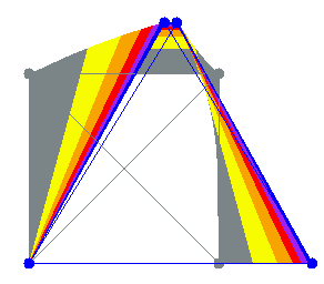
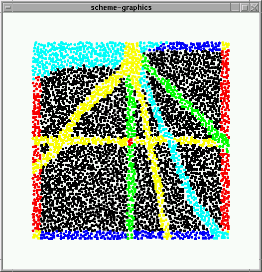
FIGURE: (a) single active cell (b) folding a sheet of cells (c) The abstract sheet where each dot represents a cell, and the green cells contract to fold the sheet in half
In order to simulate non-regular cell placement and large numbers of cells, an abstraction of the mechanical model is used. Theprogrammable flexible sheet consists of thousands of randomly but densely distributed cells. It implements onlyone type of mechanical operation: flat folding. In the mechanicalmodel, the crease width must be many cells wide in order to fold thesheet. Also cells contract only the fibers that are perpendicular to the crease orientation. In the abstract sheet, the creases must also fulfill these requirements.
(a)(b)
(c)
FIGURE: (a) single active cell (b) folding a sheet
of cells (c) The abstract sheet where each dot represents a cell, and the
green cells contract to fold the sheet in half
| Gradients | value increases with distance; always travels over the whole distance of the sheet; send-gradient and received-gradient? ; biological analog= chemical gradients used during embryogenesis |
| Tropism | ability to find the neighbor with the lowest gradient value; used to implement growing a towards a point; biological inspiration = neurons following chemical paths, plant stems growing towards sunlight |
| Comparator | can compare two gradient values to see if they are equal; biological analog = head-thorax-abdomen partitions during fruit fly embryogenesis |
| Contact | make contact with cells that touch as a result of folding; biological inspiration = epithelial cell behavior (multiple layer skin - can act as a single thick skin or individual layers) |
| Seep thru
(Example) |
gradient values can seep through contact neighbors, therefore the gradient value approximates euclidean distance from the source, rather than distance along the unfolded sheet; biological inspiration = epithelial cell sheet behavior |
| Induction | Each cell has an apical (top) and basal (bottom) surface; induction allows one cell to induce its polarity on another cell through contact; biological inspiration = tissue induction where one region of cells induces its type or function or polarity on new cells that it comes into contact with. |
Each of the primitive operations (pops) can be implemented using the amorphous primitives. The implementation of a pop can be expressed in many ways - as a procedure that checks events, using coore's ECOLI like message handlers or as a set of rules in ron's dna language. Here I have expressed them as a set of rules similar to ron's dna language (and nancy lynch's io automata). Each rule is written as a tuple - (event, condition, action-list). A rule is executed atomicly, but the rules are not ordered within the set.
As with most amorphous computors, all cells execute the same program
in parallel, have their own local state and are not synchronized. In addition
each cell has code that implements the creation and propogation of gradients
as well as code for collecting values from neighboring cells and transferring
control to a neighboring cell (tropism). Each cell can also detect neighbours
that its comes into contact with as a result of a fold.
| (fold-onto p1 p2)
Huzita's axiom 2: Given two points p1 and p2, we can fold p1 onto p2. This results in a crease line that bisects the line p1p2 at right angles. Any point on the crease line is equidistant from both p1 and p2. If the cells belonging to p1 and p2 generate two chemical gradients then all other cells can compare if the gradient levels are the equal. If so then they belong to the new crease line. |
 |
| (axiom2-ruleset p1 p2 g1 g2)
(start
(start
((and (recvd g1) (recvd g2))
((and (recvd g1) (recvd g2))
|
; start event
; (recvd g1) is an event that is generated when the cell has
received
; The width of the crease line depends on the definition of "equal";
|
| (fold-line p1 p2)
Axiom 1: Given two points p1 and p2, we can fold a line through them. The crease line is a line from p1 to p2. This is achieved using the idea of tropism and growing points (see coore thesis). The cells belonging to p2 generate a gradient gstart. When the gradient arrives at the group of cells representing p1, the cell with the lowest gstart value starts the crease line. It then collects its neighbors values for gstart and selects the neighbor with the lowest value to continue the crease line. Thus the crease line grows towards p2. When it reaches any cell belonging to p2, that cell creates a new gradient gend, signalling the successful completion of the crease line to all cells. |
  |
| (axiom1-ruleset p1 p2 gstart gend)
(define head #f)
(start
((recvd gstart)
((recvd 'new-head)
((recvd 'new-head)
((recvd 'new-head)
((recvd gend)
|
; local variables ; all p2 cells start the gradient
; Upon recieving gstart
; Upon receiving a new-head msg
; all nbrs of a head cell are part of the crease
; when the crease arrives at a p2 cell, the
The actual local rules are slightly more
|
| (fold-lontol l1
l2)
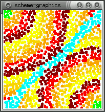
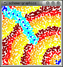
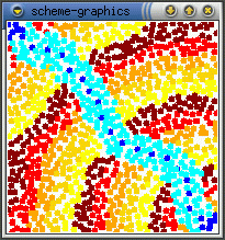
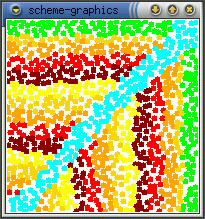
Axiom 3: Given two lines l1 and l2 we can fold l1 onto l2. The crease line is a bisector of the angle between l1 and l2. Any point on the crease line is equidistant from both input lines and we can actually implement this with the exact same ruleset as axiom2 fold-onto but passing in lines instead of points. There is one problem with this axiom. In certain cases, two crease lines can be generated. This is happens when the intersection of l1 and l2 lies more within the sheet and happens because a) when two lines cross (X) there are two bisector lines and b) the gradient can curve in a weird way around the end of a line. The picture on the left shows this happening - a fold-lontol of l1 and l2 (green lines) results in the cyan lines. In cases where this happens one needs to use regions to restrict the crease to form in the correct quadrent. |
 |
| (fold-onto-self p1 l1)
Axiom 4: Given p1 and l1, fold l1 onto itself such that the crease goes through p1. The crease line is a line perpendicular to l1 that passes through p1. This can be achieved by growing a line towards l1 (green) from p1. This uses the same ruleset as axiom1 except that the first argument is a point. |
 |
(intersect l1 l2)
(start
(start
(and l1 l2)
(not (and l1 l2))
((done #t)))
((done #f)))
(seepthru true/false)
This changes the behavior of the runtime system that implements gradients
and send-msg. If seep through is set to true, then gradients values can
seep thru neighbors that are in contact and send-msg broadcasts both to
neighbors within the sheet as well as contact neighbors. For the most part
the rulesets remain the same.
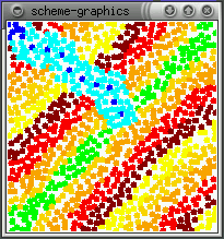
The real effect of seepthru is on how distance is interpreted. Without seep thru (a,b), the gradient approximates the euclidean distance along the sheet's surface, the fold is irrelevant. With seep thru: (c,d), the gradient approximates the euclidean distance on the folded sheet. (b,d) show what the gradient looks like when the sheet is unfolded.
(a) 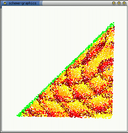 (b)
(b)  (c)
(c) 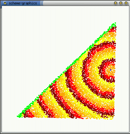 (d)
(d) 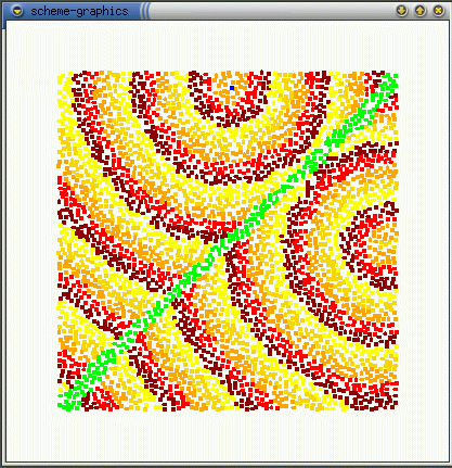
Note: The image in (d) reminds me of butterfly wings. This might be
how the perfectly symmetric wing images are produced - the winges are folded
together when the pattern forms and it seeps through both wings. When the
wings are opened (unfolded) then you get perfect mirror images (as opposed
to some complex reaction diffusion boundery idea). This idea can be used
to generating large scale geometric patterns - tesselations, triangulations
- by folding and is somewhat akin to how one can create snowflake shapes
by repeatedly folding a paper and making a few cuts. Idea is explored further
in the results section.
(execute-fold l1 type landmark)
The implementation of this is based on activecell
dynamic simulations. Each cell squeezes the appropriate apical or basal
fibers to create the fold. When all the cells in the crease squeeze their
apical fibers, the sheet folds up and if the cells squeeze their basal
fibers then the sheet folds in the other direction. In the hlsim (high
level simulator) world, the fold occurs along the best-fit-line computed
from all cells that are part of l1.
Induction: The cells must coordinate to maintain a global notion of apical and basal sides of the cellsheet in order to execute folds. A crease line divides the sheet into two disjoint regions and once a fold is executed, the cells in one of those regions must change their apical basal polarity to match the other region. The landmark defines which region will have its polarity induced by the other. This is achieved by having the landmark produce a gradient that cannot pass through the crease, thus marking the cells on one side (see define-region below). This is inspired by the idea of tissue induction where one region of cells induces its type or function or polarity on new cells that it comes into contact with.
(a) 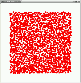 (b)
(b) 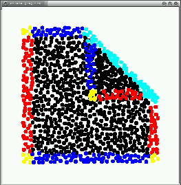 (c)
(c) 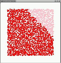
FIGURE: For each cell, red implies the apical surface
is facing upwards, and pink basal. Originally all cells have the same polarity
(a).
After making an apical fold using the top right corner
as a landmark (b), we see upon unfolding that the top region of cells
have inverted their polarity (c).
Crease Direction: as shown in the dynamics simulations of cellsheets, in order to form a fold the cells must contract fibers that are perpendicular to the direction of the crease. The question is can the cells that are in the crease locally estimate the direction of the crease and the answer is yes. If each cell computes the ratio of nbrs-in-the-crease: total-nbrs, then the cells with the maximum ratio value lie along the center of the crease. Each cell can locally estimate the direction perpendicular to the crease by looking at the nbrs with the highest and lowest ratios. Figure (a) shows cells estimating the direction of the line and (b) shows estimating the perpendiculars to the line. Seems that creases closer in width to the communication radius (orange creases) generate better estimates.
(a)  (b)
(b) 
(define-region R1 (l1 p1))
(within-region R1 ...)
A region is defined by a crease line that cuts the sheet into two disjoint
regions and a landmark that distinguishes one side of the crease from the
other. At the local level a region is created by having the landmark
create a gradient that is unable to pass through the crease - the crease
acts as a impassable boundery. The create-region rules implement both define-region
as well as apical/basal induction.
| (create-region-ruleset p1 l1 gbounded gend)
(start
((recvd gend)
|
; if p1, then initiate a gradient that cannot pass the crease l1 ; then initiate a normal gradient ; when recieve gend then check if recieved gbounded
|
Within-region restricts any operations within its scope to only occur on cells that are part of that region. This is implemented by adding a precondition on all local rules. More complicated regions can be created by oring and anding existing regions.
Note: In the current implementation, gradients used in the axioms still
travel over the whole sheet in order to maintain the self-synchronizing
nature of the axioms.A different implementation of within-region would
be to simply restrain all gradeints from moving accross the dividing crease
line - thus effectively
containing the effect of an axiom within
one region (setting up impassable bounderies).This has a cute biological
implication that the exact same ruleset, with the exact same chemical gradients,
can be used to create multiple similar structures (e.g. fingers) with different
scales and without interference simply by manipulating bounderies. Unclear
if this method is as powerful as the previous one (may not cover flaps
idea but may allow parallel execution?)
| Global Program:
(define l1 (fold-onto c1 c2))
|
Compiled Structure:
Fixed: (majority of code)
|
Synchronization: At a global level, the axioms have dependencies, therefore the cells must coordinate before moving on to the next fold. This does not require cells to be synchronous or execute in lock step (and thanks to hlsim they do not) . All that is required is that a cell start the next axiom ruleset only when its fairly sure the previous crease is done (also known as barrier synchronization).
The local rules are to a large extent self synchronizing because of the gradients. The gradients travel over the whole sheet and therefore the same gradients used for the axioms can also act as barrier synchronizers. Gradients themselves do not depend on synchronous cell behavior. In axioms 1 and 4, the end is clear when the crease reaches the end point and a signal is sent. Axioms 2 and 3 are more distributed and we use a calibration phase where a gradient is sent across the sheet twice and each cell locally times it. This gives cells local estimates of the time for the axiom completion and again the end points (cells) are responsible for sending the end gradient. Again these techniques depend on average behavior and do not ensure that every cell completed the rule sucessfully. As a result of the way gradients propogate across the sheet, there is almost always a lag accross the sheet in some direction. However the same gradient propogation tends to keep cells roughly in sync with their local neighborhood.
As shown in dynamic simulations on active cells, the cells do not all
need to fold at the same time to achieve the final folded sheet. Nevertheless
marking the end of the fold is more complicated. One way is to use contact
between sheet surfaces as an indicator of succesful folding. The cells
that make contact can create a gradient. Another method would be concensus
amongst the crease cells that they are no longer changing rapidly. This
part still needs to be proven but I believe that all the issues are solvable.
One difficulty is the fact that the abstract simulator executes the
fold at a particular moment in time, rather than it happening slowly over
time and artficially synchronizes the fold. May need to prove this part
in the dynamic simulator.
| Local State | = number of unique crease / pt identifiers (boolean) |
| Gradient Storage | = 2-3 (floating point + nametag)
Each axiom uses new gradients. Therefore once an axiom is complete, the gradient value can be thrown away and the space used for the next ones. |
| Program Storage | = mostly fixed + epsilon
The local rulesets constitute the fixed part. The sequence of folds is then simply expanded to a sequence of ruleset calls which takes very little space compared to the fixed part. (should the runtime system - low level cell capabilities such as gradient propogation and detection, neighbor communication, contact, fiber control, etc - be included in storage analysis? probably consider separately) |
| Temp State (heap) | = depends on the level of nesting, let statements and procedure calls at the high level. again mostly booleans. |
| Gradients Used | = 2-3 per axiom call.
Most gradients will travel over the whole sheet, however as the sheet gets folded smaller, the gradients travel over less distances. Gradients affect both communication and time. |
In general the reliance on gradients makes this language very communication intensive with very simple computation and low (mostly fixed) storage requirements.
Code Conservation: The majority of the local program remains the same across all global shapes and encodes the rules for each of the local primitives. The global shape is encoded in the sequence in which the primitives are called, and this forms a very small part of the local program. This gives us one possible explanation of the fact that large sections of the DNA remain the same accross different species. Futhermore simple mutations in the sequence could create whole new structures (extra fingers, wings) whereas mutations in the primitives could doom the embryo.
Reuse of Gradient Names: Although each axiom creates new gradients, once the axiom is complete the gradients are no longer needed. This means that if that state is purged from the cell at the end of an axiom the same gradient names can be used later. For example, let us say we have gradients g1-g6. The first axiom could use g1 g2 and then use g3 as the completion signal that wipes out g1 and g2 records (and g6 if any). The next axiom can use g4 and g5 and then use g6 (the copmpletion signal) to wipe out g5 g4 and g3. Now the next axiom can safely reuse g1 g2 and g3. Hence the number of distinct gradient names that need to be used can be made quite small.
In a biological system, this would seem to imply that one could reuse the same chemicals over and over to create different patterns at different times within the development. This would make it very hard for chemical probes and ideas like mapping genetic regulatory networks to illuminate the function of the chemical and the eventual structure being accomplished...
Using Regions to Limit Gradients: Gradients do not
need to travel over the entire sheet. One could create regions and then
only use gradients within that region. Similar idea to creating appendages
and organs and then limiting parts of the program to run witin that region.
In OSL one could allow different regions to execute in parallel and then
use final gradient that travels over the whole sheet to synchrnoize the
end (dataflow).