The Simulator
To study these networks of pulse-coupled oscillators, I developed a simulator in Scheme and later modified a Java simulator by Jake Beal. As always, the language is unimportant but each has its own advantages: Scheme treats functions as first class objects (quite useful in a number of situations when I was coding this simulator), while Java has much better graphical capabilities and is slightly faster. I've included this page so that anyone creating a simulator does not have to re-invent the wheel. If you are working on a simulator and have any useful or interesting ideas, or if you would like a copy of the simulator I use, please e-mail me.
Representations
Spike Train Representation
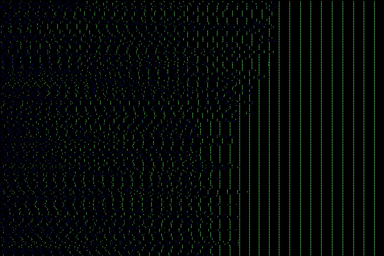
The first method of representation is called a spike train representation (from the neuronal spike trains in the literature). Each node is assigned an index, and then node index is one axis and time is the other. A point is drawn at (t,n) if node n fires at time t. If you are working on a line, ring, or a circulant graph (a ring with more connections), this representation is pretty good. Unfortunately, when working in two or more dimensions, this is a very limiting representation, as the indexing scheme must be chosen so that nodes which are close in hops are close in index, and this is impossible to do perfectly. In my simulations, I put a green dot if a node fires at the same time as one of its neighbors, and a blue dot if a node fires when none of its neighbors do.
| Node Index |
 |
| Time |
The above simulation is on a line, and it is clear when regions of the line have synchronized and when the whole line has synchronized. In large simulations of two-dimensional lattices, it is still rather clear, but in simulations of random spatial distributions with nearest neighbor coupling, it is much harder to see synchronized domains.
Direct Representation
In the direct representation, nodes are placed in their actual locations, lines are drawn between coupled neighbors (with arrows, if connections are not necessarily bi-directional), and each node has a color and a phase line. The lines between connected nodes can be different colors to represent, for example, groups when using the grouping algorithm. The color is one of two colors, representing the first portion or second portion of this phase (portions may be divided equally, or if there is a fixed point you may want to divide the period there). The color of each node is just to give you a general idea of what is going on. The phase line is a short line extending from the node, pointing in the direction of the global time of firing (we can store a global time in the simulation, even if the processors cannot have access to it) modulo 2 pi. This way, any synchronized groups will all have phase lines pointing in the same direction.
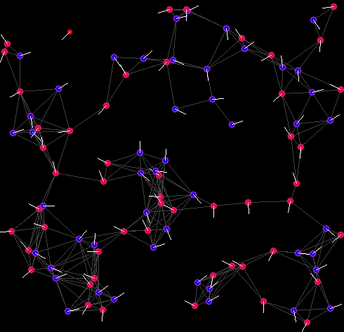
The direct representation is more intuitive, but does not give any temporal information (unless you have been watching the simulation the entire time). Obviously the state of the simulation should be written to a file (so that the simulation can be re-run later, or run with a different display, or analyzed), but it is easier to see some temporal patterns with the spike train representation. It is often much easier to see groups and borders between groups in the direct representation.
Informational Graphs
There are also various informational graphs which can give you a good idea of what is going on in the system. The simplest is the number of nodes firing at any given time. Very easy to code, and often can give you information about a large synchronized group, and it is very easy to see the rate of synchronization. The next is a graph of the largest n synchronized regions at any given time (where n is usually 1, 5, or 10, depending on the size of the simulation).
Other Details
Time
Some simulations use discrete time, and others use "real time." Discrete time has some obvious disadvantages, most notably lack of precision. Another problem which showed up was that some of the equations used underflow (are too small for Scheme or Java) when using a period of, say, 30 discrete ticks as opposed to 1 "real second." Real time is implemented by calculating the next time of an event (a processor spiking, responding to a spike, dying, starting, etc.) and then advancing the global clock (and each of the processor's clocks) to that time.
Normalization
Basically, we normalize as much as possible to [0,1]. So the area on which the processors are located is the unit square, the default period for the processors is 1. In Mirollo & Strogatz (1990) they normalize the periods to 1, but when using a spread of instrinic frequencies, this cannot be done.
Lag
There are several ways to implement lag. In general, you can attach two lag times to a spike: transmission lag (which includes processing time for the transmitting processor) and processing lag. Transmission lag means that the receiving processor has no knowledge of the spike until the transmission time has run out