6.888 Lab 3: Wireless Localization
Lab 3 Due Friday Oct. 25, 11:59 pm
Introduction
In this lab, you will learn some basic concepts on wireless localization and antenna arrays. The code for
this lab will be written in matlab. We will provide you with a skeleton code. Ideally, you will only need to
modify the places where you see : "... add your code here ..." . We will provide you with wireless signals on
which you can test your code. The lab will be divided into several tasks. Each task will require you to run some
test script which will output a file or plot a figure. You will have to keep the figures and the output files
and submit them along with your src code.
In addition to submitting your code and results, you will have to answer some questions. You can answer these questions in a .pdf file
which you should include in the .zip file which you will submit.
You can download a copy of the lab code here : 6.888_lab3.zip
The code has 4 subfolders:
- SRC_CODE: You need to implement some of these functions.
- Test_Scripts: Code to test the functions you implement.
- Mat_Files: Signals to test your code.
- Results: This folder is initially empty. The test scripts will output files in this folder
The above folders should contain the following files:
| SRC_CODE | Test_Scripts | Mat_Files | Results |
| angle_of_arrival_linear.m | test_angle_of_arrival_linear.m
test_vary_AoA_linear.m
test_vary_fc_fix_n_d.m
test_vary_d_fix_n_fc.m
test_vary_n_fix_d_fc.m | Test_AoA_Linear_R1.mat
Test_AoA_Linear_R2.mat
Test_AoA_Linear_R3.mat
Test_AoA_Linear_R4.mat
Test_AoA_Linear_R5.mat | Result_AoA_Linear.mat
Result_AoA_Linear.fig
Result_AoA_vs_fc.fig
Result_AoA_vs_d.fig
Result_AoA_vs_n.fig |
| compute_multipath_profile_linear.m | test_compute_multipath_profile_linear.m
test_mp_vs_n_linear.m | Test_MP_R1.mat
Test_MP_R2.mat | Result_MP.fig
Result_MP_vs_n.fig |
| compute_multipath_profile_sar.m | test_compute_multipath_profile_sar.m | Test_MP_SAR_R.mat | Result_MP_sar.fig |
| find_nearest_ref.m | test_manual_mp_matching.m
test_dtw_manual_mp_matching.m | Test_Localization_R.mat | Result_MP_ref1.fig
Result_MP_ref2.fig
Result_MP_dtw1.fig
Result_MP_dtw2.fig |
| compute_multipath_profile_circular.m | test_compute_multipath_profile_circular.m
test_compute_multipath_profile_circular_2.m
test_linear_vs_circular.m | Test_MP_Circular_R1.mat
Test_MP_Circular_R2.mat | Result_MP_Circular.fig
Result_MP_Circular_2.fig
Result_Linear_vs_Circular.fig |
| cdtw.m | . | . | . |
Task 1: Linear Antenna Array
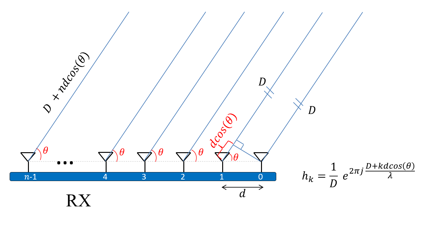
Consider the antenna array system shown in the figure above. We will assume there is a single path from the transmit antenna to
each receive antenna. Implement the function angle_of_arrival_linear.m. It should take as
input an array corresponding to the channels estimated on each antenna. It should also taks as input the number of antennas (n), the
separation distance (d) between the antennas in m and the carrier frequency (fc) in Hz. It should output the angle of arrival in
radians. If you need, you can use the builtin matlab function unwrap( ).
Run the code test_angle_of_arrival_linear.m. It will output the file
Result_AoA_Linear.mat which will contain four angles.
Q.1.1- In what direction is the transmitter relative to the receive antenna array in each of the 4 cases?
Run the code test_vary_AoA_linear.m. It will output the figure
Result_AoA_Linear.fig which shows the estimated angle as a function of the true angle.
Q.1.2- What is one limitation of using a linear array?
Run the code test_vary_fc_fix_n_d.m. It will output the figure
Result_AoA_vs_fc.fig which shows the estimated angle as a function of the carrier frequency.
Q.1.3- Assuming that the correct angle of arrival is 0.6 radians, in what frequency range does the linear array give wrong
estimates of the angle of arrival? Why does it fail for these frequencies?
Run the code test_vary_d_fix_n_fc.m. It will output the figure
Result_AoA_vs_d.fig which shows the estimated angle as a function of the separation between antennas.
Q.1.4- Assuming that the correct angle of arrival is 0.6 radians, for what separation between antennas does the linear array give wrong
estimates of the angle of arrival? Why does it fail for these separations?
Run the code test_vary_n_fix_d_fc.m. It will output the figure
Result_AoA_vs_n.fig which shows the estimated angle as a function of the number of antennas.
Q.1.5- How does increasing the number of antennas affect the estimation of the angle of arrival?
Task 2: Multipath Profiles
Recall to compute the multipath profile, you have to compute the beam strength along different angles using the following equation:

Implement the function compute_multipath_profile_linear.m. It should take as
input an array corresponding to the channels estimated on each antenna. It should also taks as input the number of antennas (n), the
separation distance (d) between the antennas in m and the carrier frequency (fc) in Hz. It should compute the multipath profile at
a resolution of 1 degree or pi/180 radians between 0 and pi (i.e. it should output 180 values).
Run the code test_compute_multipath_profile_linear.m. It will output the figure
Result_MP.fig with two subplots showing the multipath profiles from 2 different transmitters.
It will also use angle_of_arrival_linear.m to calculate the angle of arrival.
Q.2.1- In each case, how many major paths appear on the profile and in what direction?
Q.2.2- Does the angle of arrival match the direction of the paths in each case? Why or why not?
Run the code test_mp_vs_n_linear.m. It will output the figure
Result_MP_vs_n.fig with three subplots corresponding to an array with 10, 20 and 30
antennas.
Q.2.3- How does the number of antennas affect the width of the beam? Explain why this happens?
Q.2.4- Is this result in-line with your answer to Q.1.5? Why or why not?
Task 3: Synthetic Aperture

In this task, instead of using an antenna array, we use a single receive antenna moving at constant speed v to simulate a synthetic aperture.
Implement the function compute_multipath_profile_sar.m. It should take as
input an array corresponding to the estimated channels and an array of timestamps corresponding to the time at which
each channel was measured. It should also take as input the speed at which the
receive antenna is moving (v) in cm/s and the carrier frequency (fc) in Hz. It should compute the multipath profile at
a resolution of 1 degree or pi/180 radians between 0 and pi (i.e. it should output 180 values).
Run the code test_compute_multipath_profile_sar.m. It will output the figure
Result_MP_sar.fig with three subplots showing the multipath profiles from 3 different transmitters.
Q.3.1- In each case, how many major paths appear on the profile and in what direction?
Task 4: Localization
In this task, we will assume there are reference RFID tags with known positions deployed in the environment. We will localize a item
by placing an RFID tag on the item which we call the target tag and finding the nearest reference tag to our target tag. We will use the
multipath profiles to try to match the nearest tags.
Run the code test_manual_mp_matching.m. It will output two figures
Result_MP_ref1.fig and Result_MP_ref2.fig. Each figure shows the
multipath profiles of four RFID tags. The profile in red is for the target tag which we which to localize. The profiles in
blue, black and green are for the three reference tags.
Q.4.1- In each of the two figures, which of the three reference tags most matches the profile of the target tag?
Implement the function find_nearest_ref.m that takes as input the multipath profile
of the target tag and the multipath profiles of 3 reference tags and outputs a number 1, 2, or 3 which indicates which
reference tag is nearest to the the target tag. You are provided with the function cdtw.m
that take two multipath profiles and computes the dtw metric. Use the dtw metric to find the nearest tag.
Run the code test_dtw_mp_matching.m. It will output two figures
Result_MP_ref1.fig and Result_MP_ref2.fig. Each figure shows the
multipath profiles the RFID target tag and the nearest reference tag.
Q.4.2- In each figure, which of the three reference tags is nearest to the target tag?
Does this match your answer to Q.4.1? If not, what property of DTW allows it to better match multipath profiles of nearby tags?
Task 5: Circular Antenna Array
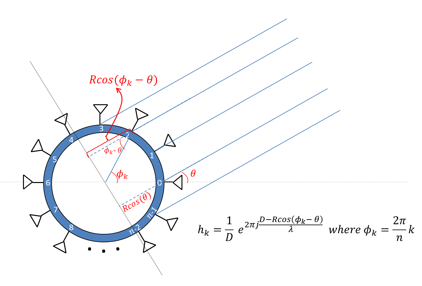
Consider the circular antenna array system shown in the figure above. Implement the function
compute_multipath_profile_circular.m. It should take as
input an array corresponding to the channels estimated on each antenna. It should also taks as input the number of antennas (n), the
radius of the array (R) in m and the carrier frequency (fc) in Hz. It should compute the multipath profile at a resolution of 1 degree or pi/180 radians
between 0 and 2pi.
Run the code test_compute_multipath_profile_circular.m. It will output the figure
Result_MP_Circular.fig with two subplots showing the multipath profiles from 2 different transmitters.
Q.5.1- In each case, how many major paths appear on the profile and in what direction?
Run the code test_compute_multipath_profile_circular_2.m. It will output the figure
Result_MP_Circular_2.fig with two subplots showing the multipath profiles of the same two transmitters
as before.
Q.5.2- In each case, how many major paths appear on the profile and in what direction?
Q.5.3- Why don't the results of Q.5.1 and Q.5.2 match? Which one is correct?
Run the code test_linear_vs_circular.m. It will output the figure
Result_Linear_vs_Circular.mat with two subplots showing the multipath profiles
from the same transmitter as captured by a linear array and by a circular array.
Q.5.4- In each case, how many major paths appear on the profile and in what direction?
Q.5.5- Based on this result, which is better the circular array or the linear array? Why?
Submit:
Submit your code via the class's submission website, located here:
https://haithamh.scripts.mit.edu:444/6.888/handin.py
You may use your MIT Certificate or request an API key via email to log in for the first time.
Compress you folder and name it lab3-handin.zip.
Upload that file to the submission website via the webpage or use curl and your API key:
$ curl -F file=@lab3-handin.zip \
http://haithamh.scripts.mit.edu/6.888/handin.py/upload