Structural Organization

Past work in Amorphous computing has focused on how to produce Structural organization in an amorphous computing medium, starting from nearly homogeneous initial conditions, and producing complicated pre-specified patterns. As an outgrowth of that effort, a number of very powerful ideas have come about in the form of programming paradigms. Most recently, Daniel Coore's Growing Point Language (GPL) has demonstrated how to configure pre-specified patterns using abstract high-level concepts such as pheremones, materials, and growing points. Growing points are processes that move from processor to processor according to a tropism. They can secrete long-range pheremone concentrations to establish a gradient field in an amorphous computing medium. As growing points travel, they label processors they visit with a material.

For example, in order to create a line segment that connects two distantly located computational elements a and b, we define two growing points, B-point and A-to-B-segment.

(define-growing-point (B-point)
  (material B-material)
  (size 0)
  (for-each-step
   (secrete+ 10 B-pheromone)))

B-point has no tropism, so it does not move, but it secretes a B-pheremone at every time step, creating a gradient field with an extent of 10 hop counts.

(define-growing-point (A-to-B-segment)
  (material A-material)
  (size 1)
  (tropism (ortho+ B-pheromone))
  (for-each-step
   (when ((sensing? B-material)
          (terminate))
         (default
           (propagate)))))

A-to-B-segment deposits A-material to every processor it visits. When A-to-B-segment detects B-pheromone, it propagates from processor to processor, with a preference for processors with higher concentration levels of the B-pheremone. Eventually, it senses the presence of the B-material and terminates.

(color
 ((B-material) "yellow")
 ((A-material) "red"))

By the time the program finishes, a red line segment should be displayed.

(with-locations
 (a b)
 (at a (start-growing-point A-to-B-segment))
 (at b (start-growing-point B-point)))

In order to specify initial conditions, specific processor id's will get bound to a and b.

These abstractions are then compiled into rules for interacting with neighbors through the Extensible Calculus of Local Interactions (ECOLI). For example, to implement a propagating growing point in ECOLI, one must imagine how the amorphous computing environment looks to a single processor. Suppose an A-to-B-segment growing point wishes to propagate. First, it must poll its neighbors for their pheremone concentrations. Then it must select a successor and notify it, so that the next processor may be activated. This process may be expressed as the Finite State Machine shown in figure

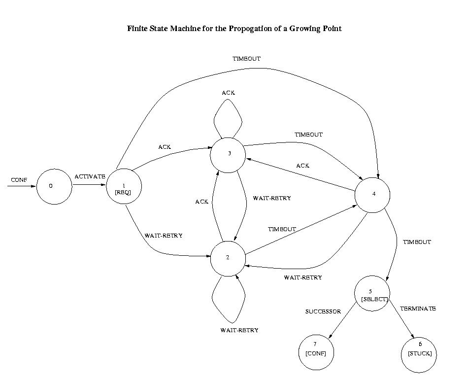
Similar Finite State Machines must be written for each primitive action of the Growing point language.

Finally, each Finite State machine is used to program thousands of processors on a High-Level Simulator (HLSIM) which emulates an amorphous computing environment where message broadcasting is unreliable, clocks are asynchronous, and the layout of processors is randomly distributed. With these tools, it has been shown that a wide variety of pre-specified patterns may be configured fairly reliably, with a reasonable chance of success. On HLSIM, the code for a line-segment produces the image shown in figure

As Amorphous Computer engineers, we are not only interested in what structures we can make, but also in how reliable we can make them.