Journal of Theoretical Biology 221: 655-664.
Erik M. Rauch, Hiroki Sayama and Yaneer Bar-Yam
Evolution in host-pathogen systems is a topic of great interest because pathogen generation times are short, and hence adaptation can occur rapidly (Anderson & May, 1982; Levin et al., 1997). There are many medically and ecologically relevant examples of pathogen evolution, such as the emergence of drug-resistant strains (Schrag & Perrot, 1996) and the decreased virulence of introduced control agents (Fenner, 1983). Host-pathogen systems are typically not well-mixed, but rather are spatially distributed. Mutant pathogen strains arise locally, and considerable variation in type is possible from one locality to another (Pielou, 1974). Moreover, host and pathogen densities are inhomogeneous and dynamic. It has become apparent in recent research that inhomogeneities in spatially distributed populations can fundamentally change the dynamics of ecological systems (Kareiva, 1990; Tilman & Kareiva, 1997), and host-pathogen systems are no exception (Mollison, 1977; Comins et al., 1992). Spatial extent can also fundamentally change evolutionary dynamics (Sayama et al., 2000). We note, in particular, that the characteristics of the pathogen can greatly affect the spatial and temporal dynamics of the host, which in turn affects the evolution of the pathogens.
There have been a number of recent theoretical studies relevant to the discussion of evolution in spatially extended host-pathogen systems (Rand et al. 1995; Boots & Sasaki, 2000; Haraguchi & Sasaki, 2000), including studies of predator-prey analogues of host-pathogen systems (Savill & Hogeweg, 1998). We will extend these studies by focusing on the dynamics and genealogy of strains. Most pathogenic species are found to consist of a number of distinct strains, distinguished from one another by a mutation or set of mutations. Our study of strain dynamics will allow us to discuss the relationship of local spatial effects and the long-term behavior of the system. In particular, we will show that mutant strains can arise that (1) increase in number rapidly over many generations; (2) are spatially clustered; (3) become extinct over longer times due to the reduction of local host densities. The evolutionary dynamics can be understood as a selection process that favors different types at different time scales.
We consider a simple spatially-extended model which allows for the mutation of a single quantitative trait, the transmissibility of the pathogen from one host to another. Similar to other recent studies (Savill & Hogeweg, 1998; Haraguchi & Sasaki, 2000; Boots & Sasaki, 2000), mutation is part of the dynamics of the model. The evolving population is composed of different types of pathogens. We will study the mechanisms that give rise to this composition.
We use a spatially extended Susceptible-Infected-Removed (SIR) model
(Sato et al., 1994; Rand et al., 1995; Andjel & Schinazi,
1996) with local reproduction of hosts. The model is a probabilistic cellular
automaton, with possible states ![]() (empty),
(empty), ![]() (susceptible host), and
(susceptible host), and ![]() (infected host). At each time step, healthy hosts reproduce into each empty
neighboring cell with probability
(infected host). At each time step, healthy hosts reproduce into each empty
neighboring cell with probability ![]() ; this occurs independently for each neighboring cell. An infected host
dies with probability
; this occurs independently for each neighboring cell. An infected host
dies with probability ![]() (virulence). Finally, an infected host
(virulence). Finally, an infected host ![]() causes a neighboring uninfected host to become infected with probability
causes a neighboring uninfected host to become infected with probability
![]() (transmissibility). The state transition probabilities are:
(transmissibility). The state transition probabilities are:
| (1) |
![]()
where ![]() is the number of uninfected host neighbors, and
is the number of uninfected host neighbors, and ![]() is the number of infected neighbors. Rand et al. (1995) note that
asynchronous updating does not significantly change the dynamics. The model
differs from that in Haraguchi et al. (2000) only in the use of discrete
time and the lack of death of susceptibles. Fig.
is the number of infected neighbors. Rand et al. (1995) note that
asynchronous updating does not significantly change the dynamics. The model
differs from that in Haraguchi et al. (2000) only in the use of discrete
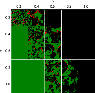
time and the lack of death of susceptibles. Fig. ![]() shows snapshots of simulations after the long-term behavior is established,
revealing how the geometry changes with differing transmissibility, virulence
and reproduction rate. The system is spatially inhomogeneous, with host and
pathogen distributed patchily. As in all host-pathogen models, the pathogen
must have a minimum transmissibility in order to propagate. In this model,
the pathogen can drive the host to extinction if it exceeds a certain transmissibility
(Sato et al., 1994). Thus, there is a minimum and maximum transmissibility
at which the pathogen and host can coexist. The region of parameter space
in which there is coexistence was obtained by Haraguchi & Sasaki (2000).
shows snapshots of simulations after the long-term behavior is established,
revealing how the geometry changes with differing transmissibility, virulence
and reproduction rate. The system is spatially inhomogeneous, with host and
pathogen distributed patchily. As in all host-pathogen models, the pathogen
must have a minimum transmissibility in order to propagate. In this model,
the pathogen can drive the host to extinction if it exceeds a certain transmissibility
(Sato et al., 1994). Thus, there is a minimum and maximum transmissibility
at which the pathogen and host can coexist. The region of parameter space
in which there is coexistence was obtained by Haraguchi & Sasaki (2000).
Rand et al. compared simulations of the spatially-extended model
with a mean field (well-mixed) version of the model. In both cases, they
considered the dynamics of a system with pathogens of transmissibility ![]() , and introduced pathogens with transmissibility
, and introduced pathogens with transmissibility
![]() (
( ![]() ). In the well-mixed version, the higher-
). In the well-mixed version, the higher-![]() population always invades, driving the lower-
population always invades, driving the lower-![]() one to extinction but itself surviving. By contrast, in the spatially-extended
version, there is a value of
one to extinction but itself surviving. By contrast, in the spatially-extended
version, there is a value of ![]() above which the mutant population does not successfully invade.
above which the mutant population does not successfully invade.
In real systems, characteristics of the pathogen can mutate, and this
must be considered when making statements about the long-term behavior of
a host-pathogen system. In order to investigate the evolutionary dynamics
of the system, mutation should be incorporated into the dynamics of the model
(Savill & Hogeweg, 1998; Haraguchi & Sasaki, 2000). The transmissibility
becomes a variable quantitative trait which is part of an infected individual's
state, rather than a global parameter. The states become ![]() ,
, ![]() , and
, and ![]() (host infected with pathogen of transmissibility
(host infected with pathogen of transmissibility ![]() ). Mutation can be introduced by assuming that there is a probability
). Mutation can be introduced by assuming that there is a probability ![]() that when a pathogen of transmissibility
that when a pathogen of transmissibility ![]() spreads, the newly infected individual has transmissibility
spreads, the newly infected individual has transmissibility
![]() :
:
![\begin{displaymath}
P(S\rightarrow I_{\tau })=\left[ 1-\prod _{\tau '}(1-\tau ')...
...}p_{\tau ''+\varepsilon }+(1-\mu )p_{\tau ''}\right) }\right]
\end{displaymath}](img17.gif)
|
(2) |
where ![]() and
and ![]() is the number of infected neighbors of transmissibility
is the number of infected neighbors of transmissibility ![]() . The assumption of incremental mutation will be extended later.
. The assumption of incremental mutation will be extended later.
Mutation causes pathogens of differing transmissibility to coexist on
the lattice. Haraguchi & Sasaki (2000) found that there is an evolutionarily
stable value of ![]() , and that this value is somewhat lower than the maximum value for which
pathogen and host can coexist. We show in fig.
, and that this value is somewhat lower than the maximum value for which
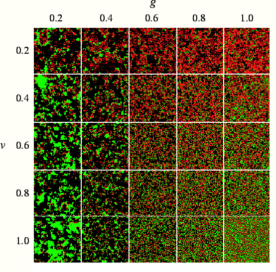
pathogen and host can coexist. We show in fig. ![]() snapshots of simulations with dynamic mutation for different combinations
of parameters. Each snapshot is taken after 10,000 generations, a time long
enough to allow the evolved transmissibility to reach a stable value, aside
from fluctuations. We find that in the presence of mutation, host and pathogen
coexist for a wide range of virulence and host reproduction rate. The evolutionarily
stable value is substantially below the maximum possible value. Fig.
snapshots of simulations with dynamic mutation for different combinations
of parameters. Each snapshot is taken after 10,000 generations, a time long
enough to allow the evolved transmissibility to reach a stable value, aside
from fluctuations. We find that in the presence of mutation, host and pathogen
coexist for a wide range of virulence and host reproduction rate. The evolutionarily
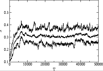
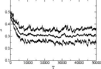
stable value is substantially below the maximum possible value. Fig. ![]() shows two typical time series of the average, minimum and maximum transmissibility
of the population. In each case, the average transmissibility is seen to
approach an evolutionarily stable value after several thousand generations,
and then stay within 5% of this value. We show in fig.
shows two typical time series of the average, minimum and maximum transmissibility
of the population. In each case, the average transmissibility is seen to
approach an evolutionarily stable value after several thousand generations,
and then stay within 5% of this value. We show in fig. ![]() a and
a and ![]() b that it will reach the same value whether the system starts with pathogens
with transmissibility above or below this value.
b that it will reach the same value whether the system starts with pathogens
with transmissibility above or below this value.
An important clue to the evolutionary dynamics of the system can be seen
in fig. ![]() , a density plot of the distribution of pathogen transmissibilities over
time. Most pathogens are within 0.03 of the evolutionarily stable value of
, a density plot of the distribution of pathogen transmissibilities over
time. Most pathogens are within 0.03 of the evolutionarily stable value of
![]() . However, there is an additional temporal structure that is apparent in
the figure: the population appears to have offshoots that persist for tens
to hundreds of generations before disappearing. These offshoots are part
of the characteristic behavior of the evolving population, even after it
has converged to the evolutionarily stable average transmissibility. In the
plot, such offshoots are most noticeable at time
. However, there is an additional temporal structure that is apparent in
the figure: the population appears to have offshoots that persist for tens
to hundreds of generations before disappearing. These offshoots are part
of the characteristic behavior of the evolving population, even after it
has converged to the evolutionarily stable average transmissibility. In the
plot, such offshoots are most noticeable at time ![]() and
and ![]() . The offshoots are visual traces of genetically related pathogens - strains.
In particular, they reflect the presence of mutant strains which substantially
exceed the evolutionarily stable value of
. The offshoots are visual traces of genetically related pathogens - strains.
In particular, they reflect the presence of mutant strains which substantially
exceed the evolutionarily stable value of ![]() , but then go extinct.
, but then go extinct.
In the remainder of this paper, we will analyze the evolutionary dynamics by examining features related to properties of strains. We will examine: (1) the reproductive success of mutant pathogens and their descendants; (2) the life histories of strains; (3) the effect of pathogen phenotype on the local environment of susceptibles; and (4) the relationship of spatial and genealogical structure. Our analysis elucidates the mechanisms by which the population comes to be dominated by strains of intermediate transmissibility. We believe similar mechanisms to be at work in many natural systems.
In order to distinguish the identity of strains, we track the genealogy of pathogens. A strain is the set of individuals descended from a single common ancestor. One can choose any ancestor, but when studying evolutionary dynamics, it is particularly useful to consider a mutant strain to begin when a mutation occurs. Mutant descendants of this first mutant can be considered the beginning of a new strain.
To obtain adequate sampling of high-transmissibility cases, which are
rare under incremental mutation because of selection, we modify the evolutionary
model given in equation 2 to have large, uniformly distributed mutations:
mutations to a random value of transmissibility between 0.2 and 1.0 with
a mutation rate ![]() ; this rate is low enough that it is rare that a mutant strain itself mutates
again. This modification does not significantly change the evolutionarily
stable transmissibility.
; this rate is low enough that it is rare that a mutant strain itself mutates
again. This modification does not significantly change the evolutionarily
stable transmissibility.
To gain insight into the reproductive success of mutants, we examine
the net reproduction ratio ![]() , which is defined as the average number of individuals infected by an infected
individual during the course of its infectious period in a population where
the infection is present.
, which is defined as the average number of individuals infected by an infected
individual during the course of its infectious period in a population where
the infection is present. ![]() has been commonly used as a measure of fitness in theoretical evolutionary
studies of host-pathogen and many other ecological systems (Fisher, 1930;
Brommer, 2000). In spatially homogeneous treatments of host-pathogen systems,
selection will tend to increase
has been commonly used as a measure of fitness in theoretical evolutionary
studies of host-pathogen and many other ecological systems (Fisher, 1930;
Brommer, 2000). In spatially homogeneous treatments of host-pathogen systems,
selection will tend to increase ![]() , and
, and ![]() increases with transmissibility (May & Anderson, 1983). The reason is
that if two pathogens have the same number of susceptible neighbors (a condition
that applies to the homogeneous version of the model), the one with the higher
transmissibility has a greater probability of infecting. On the other hand,
in the spatially distributed host-pathogen model, as we have seen, pathogens
with intermediate transmissibility dominate. This implies an anomalous feature
of the relationship between the reproductive ratio and transmissibility. The
reproduction ratio averaged over many generations has a peak at the evolutionarily
stable transmissibility. By contrast, the reproduction ratio of mutants when
they first arise is an increasing function of transmissibility.
increases with transmissibility (May & Anderson, 1983). The reason is
that if two pathogens have the same number of susceptible neighbors (a condition
that applies to the homogeneous version of the model), the one with the higher
transmissibility has a greater probability of infecting. On the other hand,
in the spatially distributed host-pathogen model, as we have seen, pathogens
with intermediate transmissibility dominate. This implies an anomalous feature
of the relationship between the reproductive ratio and transmissibility. The
reproduction ratio averaged over many generations has a peak at the evolutionarily
stable transmissibility. By contrast, the reproduction ratio of mutants when
they first arise is an increasing function of transmissibility.
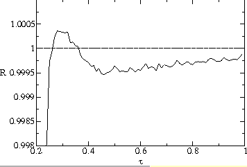
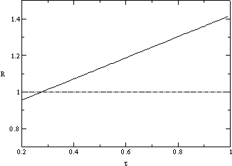
This contrast can be seen in figures ![]() a and b. Fig.
a and b. Fig. ![]() a shows
a shows ![]() averaged over many generations. For values of
averaged over many generations. For values of ![]() centered on the evolutionarily stable value of 0.3,
centered on the evolutionarily stable value of 0.3, ![]() is slightly greater than one. (A self-sustaining stable population without
mutation would have a reproduction ratio of exactly one; here the reproduction
ratio is greater than one because of mutated offspring with higher and lower
transmissibilities which have lower reproduction ratios.)
is slightly greater than one. (A self-sustaining stable population without
mutation would have a reproduction ratio of exactly one; here the reproduction
ratio is greater than one because of mutated offspring with higher and lower
transmissibilities which have lower reproduction ratios.) ![]() is significantly lower for both higher and lower values of the transmissibility.
We contrast this time-averaged value with the reproduction ratio of the initial
mutants; fig.
is significantly lower for both higher and lower values of the transmissibility.
We contrast this time-averaged value with the reproduction ratio of the initial
mutants; fig. ![]() b plots the expected number of offspring of a mutant one generation after
it arises. In this case,
b plots the expected number of offspring of a mutant one generation after
it arises. In this case, ![]() increases rapidly and roughly linearly with
increases rapidly and roughly linearly with ![]() , from a value of one at
, from a value of one at ![]() to a value of 1.4 at
to a value of 1.4 at ![]() . This must occur due to the equivalence of the environments into which all
the mutants are introduced on average. Thus, selection does not act instantaneously
to favor pathogens of intermediate transmissibility. The difference between
the time-averaged and mutant reproduction ratios points out the need to consider
the reproductive success of pathogens over the life history of a strain.
. This must occur due to the equivalence of the environments into which all
the mutants are introduced on average. Thus, selection does not act instantaneously
to favor pathogens of intermediate transmissibility. The difference between
the time-averaged and mutant reproduction ratios points out the need to consider
the reproductive success of pathogens over the life history of a strain.
Fig. ![]() plots a measurement of the average population size
plots a measurement of the average population size ![]() of a strain as a function of transmissibility
of a strain as a function of transmissibility ![]() and number of generations
and number of generations ![]() since the beginning of the strain. Strains with higher
since the beginning of the strain. Strains with higher ![]() grow much faster than ones with lower
grow much faster than ones with lower ![]() for a large number of generations. They reach a maximum and start declining
after about 30 generations and eventually go extinct. This is consistent
with both figures
for a large number of generations. They reach a maximum and start declining
after about 30 generations and eventually go extinct. This is consistent
with both figures ![]() a and b. We plot in fig.
a and b. We plot in fig. ![]() a normalized net reproduction ratio of the mutant strain over the course
of its life history
a normalized net reproduction ratio of the mutant strain over the course
of its life history ![]() , representing the average number of offspring per generation from the beginning
of the strain to time
, representing the average number of offspring per generation from the beginning
of the strain to time ![]() . This measure of reproductive success can be seen to decrease below one
for types significantly greater than the evolutionarily stable value at around
. This measure of reproductive success can be seen to decrease below one
for types significantly greater than the evolutionarily stable value at around
![]() generations. The high-
generations. The high-![]() strains can grow in the short term, but die out in the long term, despite
the fact that they have a higher net reproduction ratio for a significant
time after they are first introduced.
strains can grow in the short term, but die out in the long term, despite
the fact that they have a higher net reproduction ratio for a significant
time after they are first introduced.
Considering the reproductive success of strains as a function of time
allows one to characterize evolutionary systems in which the reproductive
success of mutants differs on different time scales. The populations of such
systems can contain a mixture of strains, each of which is successful on
a different time scale. Fig. ![]() shows the most successful type as a function of time for the host-pathogen
system.
shows the most successful type as a function of time for the host-pathogen
system.
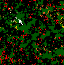
To understand the life history of strains, it is helpful to examine the
relationship of pathogen phenotype and the local environment of susceptible
hosts. Fig. ![]() shows a mutant strain
shows a mutant strain ![]() generations after it arose, with a value of
generations after it arose, with a value of ![]() that is significantly above the evolutionarily stable type. This strain
has arisen from a single ancestor at time
that is significantly above the evolutionarily stable type. This strain
has arisen from a single ancestor at time ![]() which mutated from a lower value of
which mutated from a lower value of ![]() . By time
. By time ![]() , the strain has become extinct. The figure suggests that the local environment
is significantly altered by the mutant type.
, the strain has become extinct. The figure suggests that the local environment
is significantly altered by the mutant type.
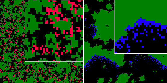
The relationship of pathogen phenotype to host geometry is apparent in
fig. ![]() , where only a single type is present in any one simulation. Fig.
, where only a single type is present in any one simulation. Fig. ![]() shows enlarged views of two panels of fig.
shows enlarged views of two panels of fig. ![]() , where it can be seen that the local configuration of susceptibles that
an average pathogen finds itself in changes with
, where it can be seen that the local configuration of susceptibles that
an average pathogen finds itself in changes with ![]() . Thus, the characteristics of the pathogen shape the characteristic geometry
of host patches that they find themselves in.
. Thus, the characteristics of the pathogen shape the characteristic geometry
of host patches that they find themselves in.
Strains that arise by mutation are generally located in an area whose
local environment has been determined by the strain it mutated from. We find,
however, that after the first mutant arises, the new strain changes the local
environment, measured by the local density, to the environment that is characteristic
of it. Fig. ![]() shows the local contact rate of susceptible hosts as a function of the
time since the strain arose, where the change can be seen to take about 40
generations. Fig.
shows the local contact rate of susceptible hosts as a function of the
time since the strain arose, where the change can be seen to take about 40
generations. Fig. ![]() shows an average over time of the local contact rate for the evolving
system and compares it with the system with only one type. We see that, for
all values of
shows an average over time of the local contact rate for the evolving
system and compares it with the system with only one type. We see that, for
all values of ![]() , the local contact rate for mixed systems (with mutation) is the same as
that for homogeneous systems (without mutation), even though in the mixed
system, many strains exist on the same lattice and individuals are constantly
mutating.
, the local contact rate for mixed systems (with mutation) is the same as
that for homogeneous systems (without mutation), even though in the mixed
system, many strains exist on the same lattice and individuals are constantly
mutating.
In order for the strains to systematically modify the local spatial structure of their environment, we expect that they are at least partially spatially segregated. To study this directly, we track genealogical distance in the following way. For each pair of individuals, the number of generations since their most recent common ancestor defines a genealogical distance between them, or coalescence time (Donnelly & Tavare, 1995). To track genealogical relatedness, we map each pair of individuals to their genealogical distance from each other. At each time step, the genealogical distances are updated so that the genealogical distance of each pair is one generation more than the genealogical distance of the respective parents of the pair. Two offspring of the same parent receive a genealogical distance of one.
We show in fig. ![]() a representation of the spatial structure of genealogical distance.
In this picture, the colors show the degree of genealogical relatedness to
a particular pathogen. The left and right panels show this for two different
individuals at the same time in an evolving population, simulated using incremental
mutations. Fig.
a representation of the spatial structure of genealogical distance.
In this picture, the colors show the degree of genealogical relatedness to
a particular pathogen. The left and right panels show this for two different
individuals at the same time in an evolving population, simulated using incremental
mutations. Fig. ![]() plots the average genealogical distance as a function of physical distance
between the two individuals in space, averaged over all pairs at that physical
distance. The genealogical distance is small for short distances, reflecting
the likelihood that nearby individuals are genetically related because of
the locality of reproduction. It increases for longer spatial distances,
indicating that strains are physically clustered on short and medium time
scales. We note that physical distance remains small for genealogical distances
of hundreds of generations. This implies that the typical lifespan of mutant
strains (200 generations) is small enough so that strains go extinct before
spreading throughout the space.
plots the average genealogical distance as a function of physical distance
between the two individuals in space, averaged over all pairs at that physical
distance. The genealogical distance is small for short distances, reflecting
the likelihood that nearby individuals are genetically related because of
the locality of reproduction. It increases for longer spatial distances,
indicating that strains are physically clustered on short and medium time
scales. We note that physical distance remains small for genealogical distances
of hundreds of generations. This implies that the typical lifespan of mutant
strains (200 generations) is small enough so that strains go extinct before
spreading throughout the space.
We have shown that the evolutionary dynamics of a generic host-pathogen model can be understood by characterizing the reproductive success of strains on different time scales. Neither spatially averaged properties nor time-averaged local properties can reveal the mechanisms responsible for the long-term composition of the population.
In particular, we have shown that: (a) the time-averaged reproduction ratio has a maximum at intermediate transmissibilities, but the reproduction ratio of mutants when they first arise increases with transmissibility; (b) the life history of high-transmissibility strains shows that they grow faster than intermediate-transmissibility ones for a significant length of time before declining and going extinct; (c) the characteristics of the pathogen determine the spatial distribution of the host, and hence the environment that the pathogens find themselves in. Strains that reproduce and grow over several generations change the local environment over time, and their local effect is the same whether or not there are other types on the lattice; (d) the genealogical distance between pathogens is correlated with their spatial distance.
In summary, we find that high-transmissibility strains change their environment in a way that is ultimately detrimental to their survival. However, there is a significant time delay before this change leads to their extinction. During this time, these strains take advantage of the host spatial structure generated by the evolutionarily stable type and are able to propagate rapidly. In this way, it is possible for strains which, by themselves, would drive the host to extinction, to be continually present in a population. In systems like the one studied, reproductive success must be thought of as a function of time. The composition of types of this, and, we believe, many natural systems, can be understood as a mixture of types, each of which is successful on a particular time scale.
| (a)
(b)

|
|
| (a)
(b)
|
| (a)
(b)
|

|
| (a)
(b)
|

|
Erik Rauch 2001-11-05