1. Bézier Curve

    1.1   Parabola
 
                   
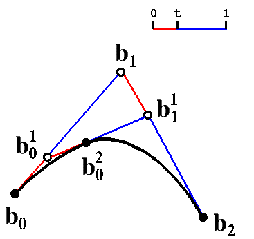
                  convex combination of the adjacent points
                   b₀¹(t) = (1-t) b₀ + t b₁
                   b₁¹(t) = (1-t) b₁ + t b₂
                               t  in    [0, 1]
             make convex combination once again
                   b₀²(t)=(1-t)b₀¹(t) + b₁¹(t)
             point b₀² goes along a curve from
                   b₀  to b₂ 
            explicit form of curve b0,2 as a function of t (parabola):

                   b₀²(t)=(1-t)² b₀  + 2t (1-t) b₁  + t² b₂ 
 

 
    1.2   Generalize to order n Bézier Curve

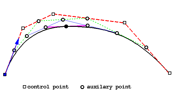
            (de Casteljau Algorithm)

            Given: points b₀ ,b₁ , ..., b_n, for any t in [0,1],
            set         b_i^r (t) = (1-t) b_i^r-1 (t) + t b_i+1^r-1 (t)
                          b_i⁰ (t) = b_i 
            Then  b₀ⁿ (t)  is the point with parameter value t on the
            Bézier curve bⁿ  .

            The polygon P formed by b₀, ..., b_n  is called the Bézier
            polygon, or control polygon of curve bⁿ .
 

                    de Casteljau scheme
 
                    b₀
               b₁   b₀¹
               b₂   b₁¹   b₀²
               b₃   b₂¹   b₁²   b₀³
 
 

     1.3   Explicit form of Bézier Curve

              Bézier curve with control points  P₀ , ...,  P_n  :
                

               Bernstein Polynomials :
 
                  

                
 
 
        Bernstein Polynomials, the cubic case (n=3) :

                           
 
      1.4     Properties of Bézier Curve
 

          1.4.1    Convex Hull Property

                   For t in [0, 1], b₀ⁿ (t)  lies in the convex hull of the control
                   polygon. This is because every intermediate point b_i^r is a
                   convex combination of points  b_i^r-1, b_i+1^r-1  .

          1.4.2    Endpoint interpolation

                               control at endpoint
                        its position,
                             first derivative,
                             second derivative, etc

             1.4.3  Shape Preservation

          1.4.4  Weistrass Theorem
 

 2.  B-Spline Curve

          2.1   Why Spline  ?

        2.2   Why Spline in Bézier Form  ?

        2.3   What is a Spline  ?
 
 

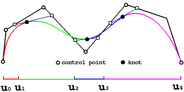
        the continuous map of a collection of intervals into 3-D space .

        each interval is mapped into a polynomial segment.
 
       2.4  C¹ and C² continuity  of  B-Spline

               C⁰  continuity(positional): curve continuous at knot point
               C¹  continuity(tangental):  curve differentiable at knot point
                 
       C²  continuity(curvature): curve doubly differentiable at knot point

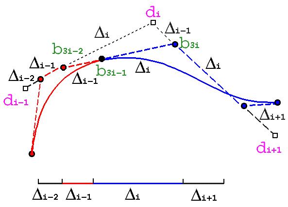
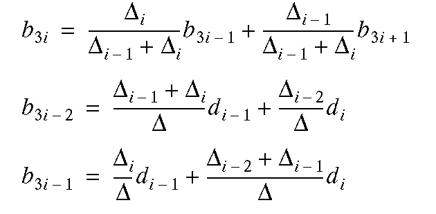
 4.   NURBS (Non-Uniform Rational B-Splines)
 
       4.1   Specify a NURB

           4.1.1    Control Points and Knots 

                  Control Points : d₀ , d₁, ..., d_L+n-1

                  Knot sequence (non-decreasing) : u₀ , u₁, ..., u_L+2n-2

                  B-Spline defined over :    [ u_n-1 ,   u_L+n-1 ]
 
 

           4.1.2    Explicit Form and Basis Functions

                if Knot Sequence becomes :  0,0,0,..,0,1,1,1,...,1
                B-Spline basis functions becomes Bernstein Polynomials .
 

       4.2   Rational Spline
 

                         equal weights
                      non-equal weights
 

                Specify weights of control points:  w₀, w₁, ...,  w_L+n-1